Amazon SQL Interview Questions

Categories:
 Written by:
Sara Nobrega
Amazon SQL Interview Questions: The Real Patterns, Traps, and Query Skills Amazon Actually Tests.
What Amazon SQL Interviews Actually Test
As the knowledge and understanding of SQL are the key requirements for both data scientists and data analysts at Amazon, many interview questions require writing solutions using this language.
In fact, Amazon asks far fewer questions about theoretical concepts and its products than other tech companies. This is why it’s crucial to practice solving SQL interview questions before an Amazon interview.
The Amazon SQL interview questions test a wide range of SQL concepts, but some notions appear in them more often. Nearly 70% of Amazon SQL interview questions concern data stores in multiple tables and ask for merging the data using JOIN clauses, Common Table Expressions, or subqueries.
Another highly prevailing concept is data aggregation using SQL functions such as COUNT() or SUM() in combination with the GROUP BY clause or using the more complicated window functions. Many questions also require data filtering and sorting using the WHERE and ORDER BY clauses.
Amazon-Style Dataset Schema
Before writing SQL, lock in the grain of each table. Most Amazon-style questions are simple once you stop mixing row levels (transaction rows vs user rows vs order rows).
In Amazon-style datasets, similar archetypes show up again and again. Let’s explore some of them.
Customers / Users table (dimension)
This is your customers-type table.
- Typical columns:
user_id(orid), name fields, city, country, signup date (sometimes) - Grain: one row per user
- What it’s for: segmentation (“by city”), cohort cuts (“new users”), deduping
Orders table (order header or order line)
This is your orders-type table.
- Typical columns:
order_id,user_id,order_date, maybetotal_order_cost, maybeorder_details - Grain warning: if there’s an
order_details/item/productfield and it varies per row, it’s often one row per order line, not one row per order.
Transactions / Purchases table (fact table)
This is the amazon_transactions / amazon_purchases vibe.
- Typical columns:
transaction_id(orid),user_id,created_at,revenueorpurchase_amt - Grain: one row per purchase event (or per transaction / line item)
- Common twist: money can be negative (returns/refunds)
Since amazon_transactions is one row per transaction, “monthly revenue” means grouping created_at by month and summing revenue. If you switch to a per-user question (like repeat buyers), you’ll usually dedupe to one row per user per day or per order first.
Amazon SQL Interview Questions (with Solutions)
Let’s start with the easier ones.
Easy Interview Questions

Amazon SQL Interview Questions #1: Workers With The Highest Salaries
Workers With The Highest Salaries
Last Updated: July 2021
Management wants to analyze only employees with official job titles. Find the title(s) of the worker(s) with the highest salary among workers who have a corresponding record in the title table. If multiple employees have the same highest salary, include all their job titles.
Data View
A quick note on what matters here:
worker.salaryholds the salary value we’re trying to maximize.title.worker_titleindicates whether someone has an “official” job title (we only consider workers who appear in this table with a non-null title).- We want job titles, not employee names, and we want all titles tied to the maximum salary.
Interview Framing (How It’s Asked + Typical Follow-Ups)
In interviews, this usually isn’t phrased as “find the max salary.” It’s framed as “Find the highest-paid employee(s) among the population that qualifies for analysis, then report a related attribute.”
The follow-up is often about scope: “Does the maximum come from all workers or only titled workers?” and “What if multiple workers tie for the maximum?” If the interviewer wants to push, they’ll ask about the ’affected_from’ column: “If titles change, which title should you use?”
A senior-sounding answer is acknowledging the decision point: “I’ll compute the max salary over only workers who have an official title, because the prompt explicitly restricts the analysis population.”
Common Mistakes (And How To Avoid Them)
A common mistake is computing MAX(salary) from worker first, then joining with title afterward. That can silently drop the max-paid worker if they don’t have a title row, and you end up returning the wrong max for the restricted population.
Another mistake is using MAX(worker_title) instead of max salary, or returning only one title by using LIMIT 1, which fails the “include all ties” requirement. If the data allowed multiple title rows per worker, failing to think about “current vs historical title” can also create duplicates or mismatched titles.
Evaluation Criteria / Rubric (How Interviewers Score It)
A strong solution makes the population restriction explicit, preserves ties, and keeps the logic readable.
A great answer computes the maximum salary over the correctly filtered population (workers with titles), returns all titles tied at that salary, and doesn’t rely on DISTINCT to patch join mistakes.
An okay answer returns the right output on clean data, but doesn’t clearly justify whether the max is computed before or after applying the “official title” constraint. A weak answer computes the max salary from all workers, drops records in the join, or returns only one title when ties exist.
Solution
1) Find the maximum salary among workers who have an official title
This subquery is the key filter that enforces the “official title only” requirement. We join worker to title so untitled employees are excluded from consideration. Then we compute MAX(w.salary) over that restricted set.
2) Pull all job titles whose worker salary equals that maximum
Now we join worker and title again so we can return the actual titles. We keep only rows where the worker’s salary equals the maximum salary computed above. If multiple employees share the same highest salary, this filter naturally includes all of them (and therefore all of their titles).
Output
| best_paid_title |
|---|
| Asst. Manager |
| Manager |
Amazon SQL Interview Questions #2: Total Cost Of Orders
Total Cost Of Orders
Last Updated: July 2020
Find the total cost of each customer's orders. Output customer's id, first name, and the total order cost. Order records by customer's first name alphabetically.
Data View
This is a “looks trivial” aggregation, but interviewers are usually checking whether you notice the grain shift. orders are multiple rows per customer, so the only correct way to get “total cost per customer” is to collapse to one row per customer with a GROUP BY.
Also, notice the prompt says “each customer’s orders,” which implies you’re summarizing at the customer level, not per order, not per day.
Grain (what one output row means): one row per customer who has at least one order in orders (with this solution).
Interview Framing (How It’s Asked + Typical Follow-Ups)
In interviews, this often comes as “roll up the fact table to the dimension grain,” and the follow-up is almost always about inclusivity: “Do you want customers with zero orders?”
If they do, you’ll need a LEFT JOIN from customers and COALESCE(SUM(...), 0). Another common follow-up is about what you’re allowed to group by: “Is first_name unique?” If not, you’d group by ’id’ from customers (and select the name as a dependent attribute).
Common Mistakes (And How To Avoid Them)
The most common mistake is grouping by first_name only. That merges different customers who share a name and produces a total that looks reasonable but is wrong.
Another mistake is selecting columns that aren’t grouped or aggregated (or “fixing” it with DISTINCT, which hides the grain problem instead of solving it). People sometimes also order by the sum instead of by first_name, which does not follow the prompt.
Validation Checks
A quick check is that the output should have one row per customer (for customers with orders), so the number of rows should match the number of distinct cust_id values present in orders.
Another check is that the total of your per-customer sums should equal the total revenue in orders over the same rows, if those don’t match, you likely duplicated rows via a bad join.
Finally, spot-check a customer you can compute mentally (like a customer with one order): their total should equal that single total_order_cost.
Solution
1) Start by joining orders to customers
We first need the customer details (like first_name) alongside each order. The join happens on customers.id = orders.cust_id. At this stage, we’re not aggregating yet, just creating the combined dataset.
2) Aggregate order costs per customer
Now that each order is linked to a customer, we can sum up spending per customer. We group by the customer columns we want to return (id and first_name). This produces one row per customer with their total cost.
3) Final query: add sorting by first name (complete solution)
The question asks us to order records alphabetically by the customer’s first name. So we keep the aggregation exactly the same and simply add ORDER BY customers.first_name ASC. This final query is the full solution.
Output
| id | first_name | sum |
|---|---|---|
| 12 | Eva | 205 |
| 3 | Farida | 440 |
| 5 | Henry | 80 |
| 7 | Jill | 535 |
| 1 | Mark | 275 |
| 15 | Mia | 540 |
| 4 | William | 140 |
Amazon SQL Interview Questions #3: Workers by Department Since April
Workers by Department Since April
Find the number of workers by department who joined on or after April 1, 2014.
Output the department name along with the corresponding number of workers.
Sort the results based on the number of workers in descending order.
Data View
This is a single-table aggregation with a date filter.
The “scenario” part is simple: you’re counting headcount by department for a time-bounded cohort (“joined on or after”). The main thing to get right is the boundary condition and the output grain.
Grain (what one output row means): one row per department in the result set.
Interview Framing (How It’s Asked + Typical Follow-Ups)
In interviews, this is often framed as “give me a breakdown by category for a cohort,” and the follow-up is usually about the boundary: “Is April 1 inclusive?” (the prompt says “on or after,” so yes).
Another common follow-up is whether departments with zero workers should appear; in this question, they won’t, because we’re grouping only over workers who meet the filter.
Common Mistakes (What Candidates Do Wrong + How To Avoid)
The most common mistake is using > instead of >= and accidentally excluding workers who joined exactly on 2014-04-01.
Another is grouping by too much (like department, joining_date), which changes the grain into daily counts. People also sometimes sort alphabetically by department instead of sorting by the computed count, which fails the prompt.
Evaluation Criteria / Rubric (How Interviewers Score It)
A strong answer applies the correct inclusive date filter, groups at the correct grain (department), and sorts by count descendingly.
An okay answer gets the right departments but doesn’t follow the sorting requirement, or uses a CTE when it isn’t needed (not wrong, just extra).
A weak answer changes the grain by grouping on unnecessary columns, or misinterprets the date boundary, and returns the wrong counts.
Solution
1) Filter only workers who joined on or after April 1, 2014
We start by narrowing the dataset to only the workers we care about. This keeps the next steps clean and avoids mixing in earlier join dates. Using a CTE here makes the query easier to read.
2) Count workers per department
Now that we have only qualifying workers, we group them by department. COUNT(worker_id) gives us how many workers are in each department. At this stage, we’re producing one row per department.
3) Final query: add sorting by number of workers (complete solution)
The final requirement is to sort departments by worker count in descending order. We keep the same aggregation and simply add ORDER BY num_workers DESC. This gives the final ranked result.
Output
| department | num_workers |
|---|---|
| Admin | 4 |
| Account | 1 |
| HR | 1 |
Medium Interview Questions

Amazon SQL Interview Questions #4: Finding User Purchases
Finding User Purchases
Last Updated: December 2020
Identify returning active users by finding users who made a second purchase within 1 to 7 days after their first purchase. Ignore same-day purchases. Output a list of these user_ids.
Data View
This table is an event log at the transaction level. A single user can have multiple purchases on the same day, which matters because the prompt is about “first purchase date” and “second purchase date,” not “first two rows in the table.”
- Grain (what one output row means): one row per qualifying
user_id. - What the table implies: multiple rows per user per day are possible, so you need to decide whether “purchase” means “transaction” or “purchase day.” The solution treats it as distinct purchase dates, which matches “ignore same-day purchases.”
Interview Framing (How It’s Asked + Typical Follow-Ups)
This is typically framed as a retention metric: “Who comes back within a week?”
The follow-ups are usually about definitions: “Are multiple purchases on day 1 considered returning?” (prompt says ignore same-day, so no), “Do we care about the second transaction or the second day with activity?”, and “What if the second purchase is 20 days later but there’s also one on day 3?” In other words, interviewers are testing whether you can lock the definition of “second purchase” before you start coding.
Trade-Offs / Decision Rules (Why This Approach vs Alternatives)
The key decision is to dedupe to one row per user-day first. That makes “ignore same-day purchases” automatic, because multiple transactions collapse into a single purchase_date.
From there, using ROW_NUMBER() to label the first and second purchase dates is straightforward and readable in an interview.
An alternative is MIN() for the first date and then MIN(purchase_date) FILTER (WHERE purchase_date > first_date) for the second date (dialect-dependent), or a self join to find the earliest later purchase.
The window approach is usually easiest to explain out loud: “I’m ranking purchase days and grabbing the first two.”
Edge Cases (Assumptions + What Breaks the Solution)
If a user has two purchases on the same calendar day only, they should not qualify: deduping to user-day enforces that.
If a user has purchases on many days, you still only care about the second distinct day, not “any purchase within 7 days.” This is subtle: a user who buys on day 1, then day 20, then day 3 doesn’t exist chronologically, but if your query isn’t careful, you can accidentally check “any later purchase within 7 days” rather than the second purchase day.
Finally, timezone can matter if created_at is a timestamp; casting to date assumes the business definition of “day” matches the database timezone.
Solution
1) Remove same-day duplicates by keeping unique purchase dates per user
First, we convert created_at into a date and use DISTINCT so multiple same-day purchases count as a single purchase day. This is important because the prompt explicitly says to ignore same-day purchases. The result is a clean set of (user_id, purchase_date) pairs.
2) Rank purchase dates per user to identify first vs second purchase
Now we assign an order to each purchase date using ROW_NUMBER(). The earliest purchase date per user gets rn = 1, and the next one gets rn = 2. This makes it easy to pick out the first two purchase days for each user.
3) Final query: extract first/second dates and filter to 1-7 day returning users (complete solution)
Next, we pivot the first two ranked rows into two columns: first_date and second_date. We filter out users who don’t have a second purchase day (second_date is NULL). Finally, we compute (second_date - first_date) and keep only those between 1 and 7 days.
Output
| user_id |
|---|
| 100 |
| 103 |
| 105 |
| 109 |
| 111 |
| 114 |
| 117 |
| 122 |
| 130 |
| 131 |
| 133 |
| 141 |
| 143 |
Amazon SQL Interview Questions #5: Top-Rated Support Employees
Top-Rated Support Employees
Last Updated: May 2023
You're analyzing employee performance at a customer support center. Management wants to identify which support agents are providing the best customer experience based on satisfaction scores.
Rank employees by their average customer satisfaction score for resolved tickets. Return the top 3 ranks, where ranks should be consecutive and should not skip numbers even if there are ties. For example, if the scores are [4.9, 4.7, 4.7, 4.5], the rankings would be [1, 2, 2, 3].
Return the employee ID, employee name, average satisfaction score, and employee rank.
Data View
This is a ticket-level table. Each row is a support ticket with a status and an optional satisfaction score. The prompt quietly enforces two filters: you only score employees on resolved tickets, and you must ignore null satisfaction scores. The output grain is employee-level.
- Grain (what one output row means): one row per employee, with their average satisfaction over qualifying tickets, plus a rank.
Interview Framing (How It’s Asked + Typical Follow-Ups)
This usually shows up as “Who are our top performers?” but the follow-ups are where the question becomes interview-grade.
Common follow-ups include: “Do unresolved or escalated tickets count?” (here, no, only resolved), “What do you do with missing satisfaction scores?” (exclude them), and “How do you rank with ties without skipping rank numbers?”
That last line is the real requirement: they’re pushing you toward DENSE_RANK() rather than RANK().
Trade-Offs / Decision Rules (Why This Approach vs Alternatives)
The clean decision rule is to separate the problem into two stages: compute a stable employee-level metric first (average satisfaction), then rank those averages. That keeps the grain controlled and avoids ranking ticket rows by accident.
For ranking, DENSE RANK is the right fit because the prompt explicitly says ranks should not skip numbers under ties. RANK() would skip (e.g., 1, 2, 2, 4), which violates the requirement. ROW_NUMBER() would force a unique ordering even when there is an average tie, which is also not what they asked.
Evaluation Criteria / Rubric (How Interviewers Score It)
A strong answer filters to resolved tickets, excludes null satisfaction values, aggregates to employee-level correctly, uses DENSE_RANK() (not RANK()), and returns all employees whose rank is within the top 3 ranks (including ties at rank 3).
An okay answer gets the averages right but uses the wrong ranking function, or returns only three employees instead of “top 3 ranks.” A weak answer ranks ticket rows directly, includes unresolved/escalated tickets, or treats null satisfaction as zero, and drags averages down silently.
Solution
1) Compute average satisfaction per employee (resolved tickets only)
We first filter the table to include only tickets that were resolved. Then we exclude null satisfaction scores so they don’t distort the average. Finally, we group by employee and compute AVG(customer_satisfaction).
2) Rank employees by average satisfaction using DENSE_RANK()
Now that we have one row per employee, ranking becomes straightforward. We use DENSE_RANK() so ties share the same rank and the next rank doesn’t skip numbers. This matches the requirements, such as [4.9, 4.7, 4.7, 4.5] -> [1, 2, 2, 3].
3) Final query: return only top 3 ranks (complete solution)
Finally, we filter to keep only employees whose dense rank is 1, 2, or 3. This automatically includes all employees tied within those ranks. The output includes exactly what the prompt asks for: id, name, average score, and rank.
Output
| employee_id | employee_name | avg_satisfaction | employee_rank |
|---|---|---|---|
| EMP-201 | Alice Johnson | 5 | 1 |
| EMP-207 | Grace Hill | 4.5 | 2 |
| EMP-203 | Carol Lee | 3 | 3 |
| EMP-209 | Ivy Scott | 3 | 3 |
Hard Interview Questions

Amazon SQL Interview Questions #6: Monthly Percentage Difference
Monthly Percentage Difference
Last Updated: December 2020
Given a table of purchases by date, calculate the month-over-month percentage change in revenue. The output should include the year-month date (YYYY-MM) and percentage change, rounded to the 2nd decimal point, and sorted from the beginning of the year to the end of the year. The percentage change column will be populated from the 2nd month forward and can be calculated as ((this month's revenue - last month's revenue) / last month's revenue)*100.
Data View
This is transaction-level revenue. Each row is a purchase event with a created_at date and a value. The key move is that the metric is at the month level, so you need to roll up to one row per month first, then compare each month to the prior month.
Grain (what one output row means): one row per month.
Interview framing (how it’s asked + typical follow-ups)
In interviews, this is typically framed as “compute MoM growth” or “build a monthly KPI trend with deltas.”
The follow-ups are usually about definitions: “Do we bucket by calendar month in UTC or local time?” and “What happens in the first month?” (no prior month, so NULL). If the interviewer wants to push, they’ll ask what you do when the prior month's revenue is zero, because the formula would divide by zero.
Trade-Offs / Decision Rules (Why This Approach vs Alternatives)
The decision rule is: aggregate monthly revenue first, then use a window function (LAG()) on the monthly totals. That keeps the logic readable and avoids self-joining the monthly table to itself.
You can compute the month key as a string (TO_CHAR) or as a real date (first day of month via date_trunc('month', created_at)), then format at the end. Using a date-month key is often safer because it preserves true chronological ordering, while strings can bite you if formatting is inconsistent.
The provided solution is ordered by the same YYYY-MM string it groups by, which works because the format is fixed-width and lexicographically sortable.
Evaluation Criteria / Rubric (How Interviewers Score It)
A strong solution produces exactly one row per month, uses LAG() to access prior month revenue, applies the formula correctly, and returns NULL for the first month. It also sorts chronologically and rounds to 2 decimals.
An okay solution gets the numbers right but has fragile ordering (e.g., ordering by month name or by a non-sortable string), or it repeats the same LAG(...) call multiple times without making the intent clear.
A weak solution computes daily deltas instead of monthly, compares the wrong months, or calculates percent change incorrectly (common sign errors or dividing by the current month instead of the prior month).
Common Mistakes (What Candidates Do Wrong + How To Avoid)
A common mistake is applying LAG() directly on raw transaction rows. That gives you the previous transaction, not the previous month’s total, so the percent change becomes meaningless.
Another mistake is grouping by MONTH(created_at) without including the year, which merges January 2019 and January 2020 into the same bucket. People also often forget to handle the first month (they try to force a value instead of leaving it NULL), or they write the percent formula as (this - last) / this, which produces a different metric.
Edge Cases (Assumptions + What Breaks the Solution)
If the prior month’s revenue is zero, the percent change is undefined (division by zero). In real pipelines, you’d usually return NULL, infinity, or define a business rule (e.g., treat as 100% if this month > 0).
Missing months are another edge case: if a month has no transactions, it won’t appear unless you generate a calendar table. The window function will then compare non-adjacent months (e.g., March compared to January), which may or may not match the business definition of “month-over-month.”
Solution
1) Aggregate revenue to the monthly level (one row per month)
2) Bring in last month’s revenue using LAG() (window function)
Now we add a window function so each month can “see” the revenue from the previous month. LAG(monthly_revenue) shifts the monthly revenue down by one row in chronological order. This step sets us up to calculate month-over-month change cleanly without a self-join.
3) Final query: calculate the MoM % change and round (complete solution)
Finally, we compute the percentage change using the formula in the prompt. We round it to 2 decimals using ROUND(..., 2). The first month will naturally have a NULL percentage change because there’s no “previous month” to compare against.
Output
| year_month | revenue_diff_pct |
|---|---|
| 2019-01 | |
| 2019-02 | -28.56 |
| 2019-03 | 23.35 |
| 2019-04 | -13.84 |
| 2019-05 | 13.49 |
| 2019-06 | -2.78 |
| 2019-07 | -6 |
| 2019-08 | 28.36 |
| 2019-09 | -4.97 |
| 2019-10 | -12.68 |
| 2019-11 | 1.71 |
| 2019-12 | -2.11 |
Amazon SQL Interview Questions #7: Exclusive Amazon Products
Exclusive Amazon Products
Find products which are exclusive to only Amazon and therefore not sold at Top Shop and Macy's. Your output should include the product name, brand name, price, and rating.
Two products are considered equal if they have the same product name and same maximum retail price (mrp column).
Data View
The important modeling detail is the equality rule: “same product” is defined by the pair (product_name,mrp), not by URL, not by price, not by brand. That means you’re doing a set difference problem on a composite key.
- Grain (what one output row means): one row per Amazon product that does not have an equivalent entry (by
product_name+mrp) in TopShop or Macy’s.
Interview Framing (How It’s Asked + Typical Follow-Ups)
In interviews, this is usually framed as “find exclusives” or “dedupe across sources,” and the follow-ups are where people lose points: “What does ‘same product’ mean?”, “Do we compare by name only or name + MRP?”, and “If Macy’s lists the same product twice, does it matter?”
Those questions are a hint that the core skill is choosing the right join key/comparison key before you write SQL.
A common follow-up is portability: “Would you solve this with NOT IN, NOT EXISTS, or an anti-join?” Because the correctness depends on null behavior and key definition.
Trade-Offs / Decision Rules (Why This Approach vs Alternatives)
The provided solution uses a tuple NOT IN against a union of competitor keys. That’s concise and reads like the business requirement: “keep Amazon rows whose (name, mrp) pair is not present elsewhere.”
In practice, many people prefer NOT EXISTS (or a left anti-join) because NOT IN can behave unexpectedly if the subquery contains nulls. If product_name or mrp can be null in the competitor catalogs, a single null can make the NOT IN filter out everything, depending on dialect and query shape.
So the decision rule is: NOT IN is fine if the key columns are guaranteed non-null; otherwise, NOT EXISTS is the safer interview choice.
Edge Cases (Assumptions + What Breaks the Solution)
The biggest edge case is nulls in the comparison key. If any competitor row has product_name or mrp null, the tuple NOT IN can become unreliable.
Another edge case is normalization: if two retailers format names differently (“Calvin Klein Women’s…” vs “Calvin Klein Womens…”), they won’t match even if they are conceptually the same product.
This question explicitly avoids fuzzy matching by defining equality as exact product_name + mrp. Finally, duplicates don’t change the logic here because you’re comparing set membership, not counts, but you still want DISTINCT on the competitor key list to keep the subquery smaller.
Validation Checks (Fast Sanity Tests)
A quick correctness check is to take a couple of returned Amazon products and search for the same (product_name, mrp) pair in the TopShop and Macy’s tables; there should be zero matches.
Then pick a known overlapping product from Macy’s or TopShop and confirm it does not appear in the Amazon-exclusive output. If the result set is unexpectedly empty, the first thing to test is whether competitor keys contain nulls: rewrite using NOT EXISTS and compare counts to diagnose null-related behavior.
Solution
Let’s code our logic.
1) Build the list of product keys sold at Macy’s or TopShop
We first extract only the comparison keys: product_name and mrp. UNION ALL combines both retailer lists into one dataset (duplicates don’t really hurt, but we can DISTINCT later). This gives us “everything that exists outside Amazon,” according to the equality definition.
2) Deduplicate that competitor key list (so matching is clean)
Now we wrap the union and select DISTINCT to get a unique set of (product_name, mrp) pairs. This avoids repeated keys showing up multiple times if the same product appears in multiple rows. The result is the exact list we want to exclude from Amazon.
3) Final query: return Amazon-only products (complete solution)
Finally, we select products from Amazon and exclude anything that appears in the competitor key set. The (product_name, mrp) NOT IN (...) check matches your equality rule exactly. Then we return the required Amazon columns: product_name, brand_name, price, and rating.
Output
| product_name | brand_name | price | rating |
|---|---|---|---|
| Calvin Klein Women's Bottoms Up Hipster Panty | Calvin-Klein | $11.00 | 4.5 |
| Wacoal Women's Retro Chic Underwire Bra | Wacoal | $60.00 | 4.4 |
| Calvin Klein Women's Carousel 3 Pack Thong | Calvin-Klein | $19.99 | 4 |
| b.tempt'd by Wacoal Women's Lace Kiss Bralette | b-temptd | $11.65 | 4 |
| Wacoal Women's Front Close T-Back Bra | Wacoal | $46.00 | 4.2 |
| Calvin Klein Women's Modern Cotton Bralette and Bikini Set | Calvin-Klein | $44.00 | 4.6 |
| Calvin Klein Women's 3 Pack Invisibles Hipster Panty | Calvin-Klein | $29.75 | 3.9 |
| Wacoal Womens Basic Beauty Contour T-Shirt Bra | Wacoal | $11.95 | 4.2 |
| Wacoal Women's Underwire Sport Bra | Wacoal | $65.00 | 4.3 |
| Hanky Panky Women's Vikini Panty | Hanky-Panky | $30.00 | 4 |
| Wacoal Women's Halo Underwire Bra | Wacoal | $48.00 | 4.4 |
| Wacoal Women's Basic Beauty Contour Bra | Wacoal | $55.00 | 4 |
| Wacoal Women's Retro Chic Underwire Bra | Wacoal | $60.00 | 4.5 |
| Wacoal Women's How Perfect Soft Cup Bra | Wacoal | $51.52 | 4.2 |
| Wacoal Women's Body By Wacoal Underwire Bra | Wacoal | $43.00 | 4.4 |
| Wacoal Women's How Perfect Soft Cup Bra | Wacoal | $60.00 | 4.1 |
| Wacoal Women's Retro Chic Contour Bra | Wacoal | $65.00 | 4.2 |
| Wacoal Women's Halo Strapless Bra | Wacoal | $46.00 | 4.2 |
| Calvin Klein Women's Modern Cotton Boyshort Panty | Calvin-Klein | $19.49 | 4.4 |
| Wacoal Women's Underwire Sport Bra | Wacoal | $52.67 | 4.3 |
| b.tempt'd by Wacoal Womens Ciao Bella Tanga Panty | b-temptd | $19.00 | 4.1 |
| Wacoal Women's Embrace Lace Bra | Wacoal | $44.50 | 4.3 |
| Calvin Klein Women's Naked Glamour Strapless Push Up Bra | Calvin-Klein | $28.27 | 3.9 |
| Calvin Klein Women's Perfectly Fit Lightly Lined Memory Touch T-Shirt Bra | Calvin-Klein | $41.40 | 4.3 |
| Wacoal Women's Amazing Assets Contour Bra | Wacoal | $65.00 | 3.8 |
| Wacoal Women's Sport Zip Front Contour Bra | Wacoal | $69.84 | 3.8 |
| Wacoal Women's Awareness Underwire Bra | Wacoal | $65.00 | 4.4 |
| Wacoal Women's Bodysuede Underwire Bra | Wacoal | $60.00 | 4.4 |
| Wacoal Women's Underwire Sport Bra | Wacoal | $45.50 | 4.3 |
| Wacoal Women's How Perfect Soft Cup Bra | Wacoal | $60.00 | 4.1 |
| Wacoal Embrace Lace Bikini Panty | Wacoal | $27.00 | 4.3 |
| Wacoal Women's Halo Underwire Bra | Wacoal | $34.95 | 4.3 |
| Wacoal Women's Lace Affair Bikini Panty | Wacoal | $22.00 | 4.8 |
| Wacoal Women's Awareness Underwire Bra | Wacoal | $65.00 | 4.4 |
| Wacoal Women's Basic Beauty Contour Bra | Wacoal | $55.00 | 4 |
| Calvin Klein Women's Naked Glamour Strapless Push Up Bra | Calvin-Klein | $29.99 | 3.9 |
| Wacoal Women's Retro Chic Underwire Bra | Wacoal | $48.00 | 4.4 |
| Calvin Klein Women's Perfectly Fit Lightly Lined Memory Touch T-Shirt Bra | Calvin-Klein | $46.00 | 4.3 |
| Calvin Klein Women's 3 Pack Carousel Thong Panty | Calvin-Klein | $20.99 | 4.7 |
| Wacoal Women's Retro Chic Underwire Bra | Wacoal | $48.00 | 4.4 |
| Calvin Klein Women's Sheer Marquisette Demi Unlined Bra | Calvin-Klein | $36.00 | 4.6 |
| Wacoal Women's Basic Beauty Front Close Contour Bra | Wacoal | $55.00 | 4.2 |
| Wacoal Women's Retro Chic Contour Bra | Wacoal | $52.97 | 4.2 |
| Calvin Klein Women's Perfectly Fit Lightly Lined Memory Touch T-Shirt Bra | Calvin-Klein | $40.48 | 4.3 |
| Wacoal Women's Body By Wacoal Underwire Bra | Wacoal | $39.46 | 4.4 |
| Calvin Klein Women's Standard Radiant Cotton Bikini Panty | Calvin-Klein | $9.88 | 4.4 |
| Wacoal Women's Retro Chic Underwire Bra | Wacoal | $60.00 | 4.4 |
| b.tempt'd by Wacoal Women's Ciao Bella Balconette Bra | b-temptd | $38.00 | 4.3 |
| Wacoal Women's Bodysuede Underwire Bra | Wacoal | $60.00 | 4.4 |
| Wacoal Women's Halo Underwire Bra | Wacoal | $48.00 | 4.4 |
| Wacoal Women's Embrace Lace Bra | Wacoal | $35.00 | 4.3 |
| Calvin Klein Women's Naked Glamour Strapless Push Up Bra | Calvin-Klein | $29.99 | 3.8 |
| Wacoal Womens Basic Beauty Contour T-Shirt Bra | Wacoal | $54.77 | 4.2 |
| Wacoal Women's Embrace Lace Bikini Panty | Wacoal | $27.00 | 4.3 |
| Calvin Klein Women's Sheer Marquisette Demi Unlined Bra | Calvin-Klein | $26.19 | 4.5 |
| Wacoal Womens Basic Beauty Contour T-Shirt Bra | Wacoal | $55.00 | 4.2 |
| Calvin Klein Women's Everyday Lightly Lined Demi Bra | Calvin-Klein | $38.00 | 3.8 |
| Calvin Klein Women's Bottoms Up Bikini Panty | Calvin-Klein | $8.00 | 4.3 |
| Calvin Klein Women's ID Wide Waistband Unlined Triangle Cotton Bralette | Calvin-Klein | $19.01 | 3.8 |
| Wacoal Women's Body By Wacoal Underwire Bra | Wacoal | $46.00 | 4.4 |
| Calvin Klein Women's Sheer Marquisette Demi Unlined Bra | Calvin-Klein | $27.00 | 4.6 |
| Wacoal Women's Retro Chic Underwire Bra | Wacoal | $69.99 | 4.4 |
| b.tempt'd by Wacoal Women's Ciao Bella Balconette Bra | b-temptd | $38.00 | 4.3 |
| Wacoal Women's Red Carpet Strapless Bra | Wacoal | $65.00 | 4.4 |
| Calvin Klein Women's Seductive Comfort Lift Strapless Multiway Bra | Calvin-Klein | $39.60 | 4.1 |
| Wacoal Women's Slimline Seamless Minimizer Bra | Wacoal | $65.00 | 4.3 |
| Wacoal Women's Awareness Underwire Bra | Wacoal | $55.25 | 4.4 |
| Wacoal Women's Embrace Lace Bra | Wacoal | $50.00 | 4.3 |
| Hanky Panky Women's Bare Godiva Thong Panty | Hanky-Panky | $25.00 | 4.2 |
| Calvin Klein Women's Seductive Comfort Lift Strapless Multiway Bra | Calvin-Klein | $39.60 | 3.9 |
| Wacoal Women's Halo Underwire Bra | Wacoal | $48.00 | 4.4 |
| Wacoal Women's Retro Chic Underwire Bra | Wacoal | $48.00 | 4.4 |
| Calvin Klein Women's 4 Pack Stretch Lace Bikini Panty | Calvin-Klein | $28.01 | 4.1 |
| Calvin Klein Women's Perfectly Fit Lightly Lined Memory Touch T-Shirt Bra | Calvin-Klein | $34.50 | 4.3 |
| Wacoal Women's Red Carpet Strapless Bra | Wacoal | $65.00 | 4.4 |
| Calvin Klein Women's ID Tanga Wide Waistband Cotton Panty | Calvin-Klein | $16.97 | 4.3 |
| Wacoal Women's Retro Chic Underwire Bra | Wacoal | $60.00 | 4.4 |
| Calvin Klein Women's Ombre 5 Pack Thong | Calvin-Klein | $59.99 | 5 |
| Wacoal Women's How Perfect Soft Cup Bra | Wacoal | $60.00 | 4.2 |
| Wacoal Womens Basic Beauty Contour T-Shirt Bra | Wacoal | $55.00 | 4.2 |
| Wacoal Women's Underwire Sport Bra | Wacoal | $42.90 | 4.3 |
| Wacoal Women's Retro Chic Underwire Bra | Wacoal | $60.00 | 4.4 |
| Wacoal Women's Retro Chic Underwire Bra | Wacoal | $54.60 | 4.4 |
| Wacoal Womens Basic Beauty Contour T-Shirt Bra | Wacoal | $55.00 | 4.2 |
| Wacoal Womens Basic Beauty Contour T-Shirt Bra | Wacoal | $55.00 | 4.2 |
| Calvin Klein Women's Perfectly Fit Lightly Lined Memory Touch T-Shirt Bra | Calvin-Klein | $41.40 | 4.3 |
| Calvin Klein Women's Modern Cotton Bikini | Calvin-Klein | $11.36 | 4.7 |
| Wacoal Women's Sport Contour Bra | Wacoal | $47.40 | 4.2 |
| b.tempt'd by Wacoal Women's Ciao Bella Balconette Bra | b-temptd | $21.89 | 4.3 |
| Wacoal Women's Sport Contour Bra | Wacoal | $65.96 | 4.2 |
| Wacoal Women's Bodysuede Underwire Bra | Wacoal | $60.00 | 4.3 |
| Wacoal Women's Halo Strapless Bra | Wacoal | $46.00 | 4.2 |
Amazon SQL Interview Questions #8: First Day Retention Rate
First Day Retention Rate
Last Updated: February 2022
Calculate the first-day retention rate of a group of video game players. The first-day retention occurs when a player logs in 1 day after their first-ever log-in. Return the proportion of players who meet this definition divided by the total number of players.
Data View
This dataset looks simple (just player_id and login_date), but the interview goal is whether you translate “first-ever login” into the correct baseline per player, and then avoid double-counting players who logged in multiple times.
Grain (what one output row means): one row total, a single retention_rate for the whole population.
What the table implies: multiple rows per player_id (a player can log in many times), so any join back to the raw logins can multiply rows and inflate counts if you don’t use COUNT DISTINCT.
Interview Framing (How It’s Asked + Typical Follow-Ups)
Interviewers usually phrase this as “day-1 retention” or “D1 retention,” then follow up with clarifications like “Is it exactly one day after, or within 24 hours?” and “Do multiple logins count multiple times?”
In SQL interviews, the expected interpretation is usually a calendar-day difference (since the column is a date here), and retention is a per-player event (a player is either retained or not).
A common follow-up is: “What if someone logs in multiple times on day 1?”, which is basically a test of whether you count players, not sessions.
Trade-Offs / Decision Rules (Why This Approach vs Alternatives)
This CTE approach is clean because it separates the baseline computation (first login date) from the retention check (did they show up on first_day + 1). It’s also easy to audit step-by-step.
Alternatives that are also valid:
- A correlated
EXISTS(“does a day+1 login exist for this player?”) can be simpler to read, and it avoids join-multiplication issues naturally. - Pre-aggregating to distinct (
player_id, login_date) first can protect you if the raw data has duplicates.
If you’re unsure about duplicates, default to COUNT(DISTINCT player_id) in numerator/denominator, or use EXISTS.
Evaluation Criteria / Rubric (How Interviewers Score It)
A strong answer usually hits these points: it correctly defines each player’s first-ever login date, checks for a login exactly one day after that baseline, counts retained players uniquely (not per row), keeps the denominator as all unique players, and returns a non-integer proportion (float/decimal), not truncated integer division.
Common Mistakes (What Candidates Do Wrong + How To Avoid)
A frequent mistake is counting rows instead of players after joining back to logins, which overstates retention for players with multiple logins.
Another common slip is using BETWEEN 0 AND 1 (which accidentally includes same-day logins) even though the prompt explicitly says “1 day after.” People also sometimes compute “day-1 after each login” instead of after the first-ever login, which answers a different question.
Edge Cases (Assumptions + What Breaks the Solution)
If a player’s first login is near the end of the dataset window, they might not have an opportunity to log in the next day, and this affects interpretation, but the question doesn’t mention censoring, so we include them in the denominator.
If timestamps (not dates) were used, you’d need to define whether “1 day” means “next calendar day” or “within 24 hours.” Also, if the table can contain duplicate (player_id, login_date) rows, you’ll want a distinct day-level table (or keep COUNT(DISTINCT ...)) to prevent inflation.
Solution
Let’s code our logic.
1) Find each player’s first-ever login date
We start by grouping by player_id and taking the minimum login_date. This gives us a single first_day anchor date per player. Once we have that, we can compare all other logins against it.
2) Identify players who logged in exactly 1 day after their first login
Now we join the first login dates back to the raw login table. This lets us compute login_date - first_day for each login event per player. We then filter to keep only events where the difference equals 1 day, which matches the retention definition.
3) Final query: compute retention rate as retained / total (complete solution)
Finally, we count how many distinct players satisfy the first-day retention condition and divide by the total number of distinct players. We cast the numerator to FLOAT so we get a decimal result instead of integer division. The final output is a single value: the first-day retention rate.
Output
| retention_rate |
|---|
| 0.5 |
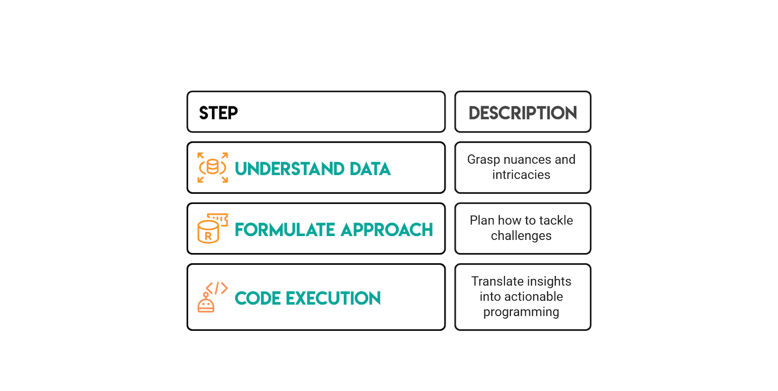
How to Solve Amazon SQL Questions (Interview Framework)
Common Amazon SQL Mistakes (and How to Avoid Them)
Amazon-style SQL interviews are designed to test whether you can work with data the way it actually exists in production: messy, full of edge cases, and requiring careful thought. Here are the most common mistakes candidates make:

1) Losing track of table grain (then patching it with DISTINCT)
This happens when you join a one-row-per-user table to a many-rows-per-user fact table without thinking through the implications. Suddenly, one customer's revenue gets multiplied by however many transactions they have, and your metrics are wildly inflated.
The solution: Always state the grain out loud before writing your joins, "this table has one row per purchase, this one has one row per user." Aggregate to the grain you need before joining, or be very deliberate about when and how you group after the join.
2) Forgetting about returns, refunds, and cancellations
Negative values in your data can throw off revenue calculations significantly. If the prompt asks you to exclude returns but you forget to filter them out, your numbers will be off or even negative.
Handle this upfront: decide whether you're including or excluding these transactions, and filter explicitly (for example, WHERE purchase_amount >= 0). Amazon prompts typically call this out directly, so read the requirements carefully.
3) Treating dates as strings
This is a subtle but common error. When you group or sort dates that have been converted to strings too early, you end up with alphabetical sorting instead of chronological, 2024-02 appearing after 2024-10, for instance.
Always use proper date/timestamp functions for grouping and sorting, and only format dates for display purposes at the very end of your query. This is especially important when output requirements specify formats such as YYYY-MM.
4) Rolling metrics without accounting for partial windows
When calculating rolling averages or other window metrics, your first few time periods often don't have complete data windows. If you're not careful, these partial windows get treated as if they're complete, skewing your results.
Follow the prompt's definition precisely. If your data starts midstream, acknowledge that early windows are incomplete and either keep them labeled as partial or filter them out, depending on what the question actually requires.
5) Window functions that appear correct but have logical errors
Forgetting to include PARTITION BY, or using a default window frame that doesn't match the question, is extremely common. You might think you're calculating a metric per user when you're actually calculating it across all users.
Always specify what you're partitioning by (user, product, time period, etc.), order by the appropriate column, and verify your logic by tracing through one example manually. Amazon interview guidance specifically highlights missing partitions as a frequent pitfall.
6) LEFT JOINs accidentally becoming INNER JOINs
This happens when you write a LEFT JOIN to preserve all rows from your left table, then add a WHERE clause that filters on the right table. That filter drops all the non-matching rows, and converts your LEFT JOIN into an INNER JOIN.
If you want to filter the right table while keeping unmatched left rows, put those conditions in the ON clause instead of WHERE. This is one of the classic interview mistakes.
7) NULL handling errors
WHERE column = NULL doesn't work, it returns nothing. NULLs also behave unexpectedly in counts, comparisons, and aggregations, often leading to incorrect results.
Use IS NULL and IS NOT NULL for comparisons, and think through what NULL actually represents in your context: unknown, not applicable, or zero. Amazon interview materials specifically call out NULL behavior as a frequent trap.
8) Confusion between WHERE and HAVING in grouped queries
Using WHERE to filter aggregate results generates an error, while filtering row-level data in HAVING can change your metrics in unexpected ways.
The rule is straightforward: row-level filters belong in WHERE, and aggregate filters belong in HAVING. This is one of those "easy to miss" mistakes that Amazon interview guides consistently highlight.
2-Week Amazon SQL Prep Plan
This plan assumes you’re practicing with Amazon-style, scenario-driven SQL questions where the real test is translating a question prompt into a clean definition (grain + constraints), then picking a pattern that survives duplicates, ties, and missing rows.
How to use this plan day-to-day
Aim for 60-90 minutes a day (or more, if you are able).
For each question, force yourself to write down (mentally or on paper) the grain and the “trap” before you touch SQL. After you solve it, do a 2-minute validation pass: row counts, spot checks, and “did I accidentally change the grain with joins?”
Week 1: Fundamentals + Amazon patterns (Easy to Medium)
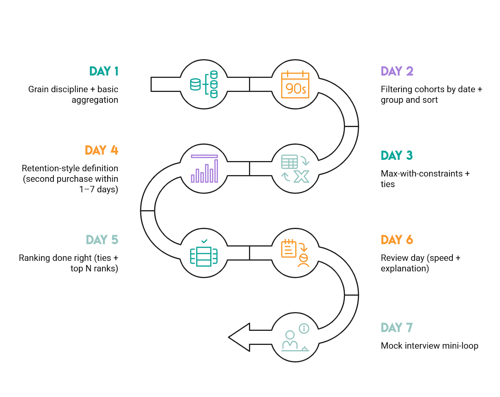
Day 1: Grain discipline + basic aggregation
Do “Total Cost of Orders” (ID 10183). Focus on grouping at the correct grain (customer) and validating totals.
Day 2: Filtering cohorts by date + group and sort
Do “Workers by Department Since April” (ID 9847). Treat it as “cohort + breakdown,” and be strict about inclusive boundaries (>=).
Day 3: Max-with-constraints + ties
Do “Workers With The Highest Salaries” (ID 10353). The key is computing the max over the qualified population (titled workers) and returning all ties.
Day 4: Retention-style definition (second purchase within 1-7 days)
Do “Finding User Purchases” (ID 10322). Lock the definition of “second purchase” (second distinct day, not second row), then implement with a clear stepwise approach.
Day 5: Ranking done right (ties + top N ranks)
Do “Top-Rated Support Employees” (ID 10554). Practice choosing DENSE_RANK vs RANK vs ROW_NUMBER and explaining why.
Day 6: Review day (speed + explanation)
Re-do Day 1-5 questions under a timer. Your goal is not new SQL, it’s cleaner reasoning: state grain, state trap, then code. If you rely on DISTINCT to “fix” duplicates, stop and re-check joins/grain.
Day 7: Mock interview mini-loop
Pick any 2 questions from the week and “talk through” your approach out loud. If you can’t explain why you chose a pattern (CTE vs EXISTS vs window), you’re not interview-ready yet.
Week 2: Advanced patterns (Medium to Hard)
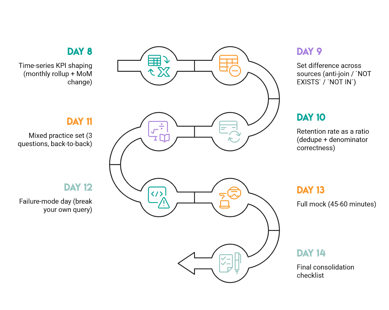
Day 8: Time-series KPI shaping (monthly rollup + MoM change)
Do “Monthly Percentage Difference” (ID 10319). The must-have habit: aggregate to the month first, then LAG the monthly totals.
Day 9: Set difference across sources (anti-join / NOT EXISTS / NOT IN)
Do “Exclusive Amazon Products” (ID 9608). Practice arguing the trade-off: NOT IN is concise but can be risky with NULLs; NOT EXISTS is safer.
Day 10: Retention rate as a ratio (dedupe + denominator correctness)
Do “First Day Retention Rate” (ID 2090). Your focus is counting players, not login rows, and preventing join multiplication.
Day 11: Mixed practice set (3 questions, back-to-back)
Do one easy + one medium + one hard from the list above. This simulates interview context switching. Keep your walkthrough structure consistent: assumptions, grain, trap, solution, and validate.
Day 12: Failure-mode day (break your own query)
Pick 2 hard-ish questions and actively try to break your solution: add a tie, add duplicates, add NULLs, remove a month, add multiple rows per key. If your query changes meaning, rewrite it in a more robust pattern.
Day 13: Full mock (45-60 minutes)
Do 2 questions under time pressure: one ranking/window question and one set logic question. Afterward, rewrite each solution to be more readable (fewer moving parts, clearer grain control).
Day 14: Final consolidation checklist
You’re ready if you can do all of this reliably: define grain first, pre-aggregate before ranking, preserve ties intentionally, choose the right anti-join pattern, and validate outputs with quick sanity checks (counts, totals, spot checks).
Practical rule of thumb for progression
Start with the Easy questions to lock in grain + aggregation discipline, move to Medium for window functions and definition traps, then finish with Hard for set logic and time-based analysis. If you’re getting stuck, it’s usually not “SQL syntax”; it's that the data definition isn’t pinned down yet.
More Big Tech SQL Interview Guides (Meta, DoorDash, Uber, etc.)
If you’re prepping for Amazon, it helps to practice on other Big Tech question styles too. The datasets change, but the patterns repeat: user activity logs, orders/transactions, time windows, and window functions.
- Meta (Facebook) SQL Interview Questions: Great for analytics-style metrics (engagement, feeds, user activity) and clean aggregation + filtering patterns.
- DoorDash SQL Interview Questions: Strong practice for marketplace-style data and messy edge cases where date logic and formatting matter.
- Uber SQL Interview Questions: Solid mix of business metrics and time-based analysis that often pushes you into window functions.
- Google SQL Interview Questions: Good when you want structured thinking and careful problem setup before writing code.
- Microsoft SQL Interview Questions: Helpful for sharpening fundamentals, plus practical query design under real constraints.
FAQs:
How hard is the Amazon SQL interview?
Amazon’s SQL questions can range from easy to medium and hard, and they tend to be practical coding problems rather than product/theory trivia.
For example, this interview question is a medium-level Amazon SQL question, while in this one, the rolling-average problem is explicitly described as hard because it requires a clear understanding of data manipulation and time-based calculations.
So, difficulty mostly depends on your comfort with multi-step business queries and careful requirements.
What SQL topics does Amazon ask most?
Nearly 70% of Amazon SQL questions involve data in multiple tables and require JOINs, CTEs, or subqueries. It also highlights aggregation (COUNT()/SUM() with GROUP BY) and “more complicated” window functions as other highly prevalent concepts.
For data engineering roles, EDA/validation, aggregation/metrics, joins, and text/datetime manipulation are also hot topics.
Do I need window functions for Amazon?
Yes! Plan to know window functions.
Amazon questions often use them, as interviewers generally expect candidates to use window functions when possible. For instance, in this interview question, the walkthrough is built around using DENSE_RANK() with PARTITION BY to rank sellers within each product category and filter the top three per group.
What’s the best way to practice Amazon SQL?
Do targeted, repetitive practice on real interview-style questions.
It is crucial to practice solving SQL interview questions before an Amazon interview. You can build your own solution based on the framework explained in this article, try other approaches, and then deliberately cover edge cases.
How long should I spend preparing?
If you already know SQL fundamentals, plan from 2 to 4 weeks of focused practice; if you’re still learning joins/CTEs/subqueries, budget closer to 2 to 3 months to reach an interview-ready intermediate level.
That longer window matters for Amazon because its SQL questions often involve multi-table merging (JOIN/CTE/subquery) and frequently use window functions.
Share