SQL Scenario Based Interview Questions and Answers

Categories:
 Written by:
Sara Nobrega
SQL scenario based interview questions to learn how to wrangle date time fields for Facebook data science interviews.
Scenario-based SQL questions are how most teams simulate real work in an interview. Instead of asking you to recite syntax, the interviewer gives you a business situation and watches how you turn an ambiguous prompt into a correct, defendable query.
That shift is intentional. SQL interviews have become more interactive and performance-focused: timed, live-coded, and closer to pair programming than a take-home worksheet. In other words, it’s rarely enough to produce “a query that runs”. You’re expected to explain why your approach is correct, how it scales, and what you’d do differently if constraints changed.
Scenario prompts also come with the same messiness you’ll see on the job: duplicates, missing events, inconsistent timestamps, or “impossible” rows that still exist because pipelines aren’t perfect. If you don’t account for those, your query might be syntactically fine and still wrong.
In this article, we’ll work through some scenario-based questions through several levels: beginner, intermediate, and advanced.
If you’re building a broader prep plan beyond scenarios, this collection of sql interview questions is a solid next stop.
Why Scenario-Based Questions Matter (and How to Answer Them Like a Senior)
Scenario-based questions are “special” because they test more than SQL mechanics.
They test whether you can reason from a vague situation to a precise data definition and then build a query that’s correct and explainable under pressure.
Interviewers like them because they can see whether you can define the metric correctly, keep row-grain under control, and choose patterns that are readable under time pressure but still scalable.
What interviewers are really testing
- Problem framing: Can you restate the question in data terms (filters, grain, joins, output shape) before you write code? That’s the difference between a fast attempt and a correct solution.
- Real-world trade-offs: Interviews increasingly reward candidates who can discuss readability vs. performance, not just output correctness.
- Handling edge cases: Messy data is normal in production, so interview questions often include it (duplicates, out-of-order events, invalid rows). Expect to clean as you query.
SQL Patterns Interviewers Test
Scenario questions aren’t really about whether you remember a function name.
They’re about whether you can take a messy prompt, turn it into a precise data definition (grain + constraints), and then choose a SQL pattern that won’t fall apart when the data has duplicates, ties, and missing rows.
Here are the patterns. All the questions we reference in this section will be shown in the SQL Scenario Based Interview Questions section.
1) Cohort logic: “must have both” (intersection patterns)
This shows up any time the prompt contains an “AND” that’s really about membership in two sets. In the Submission Types question, the trap is reading it as “Refinance or InSchool” and writing a single WHERE type IN (...) filter, which answers a different question.
What interviewers are testing: whether you translate “must satisfy both” into set logic at the right grain (usually user_id), and whether you avoid being fooled by multiple rows per user.
Typical SQL moves you’ll see:
- Build two cohorts at the same grain and
INTERSECTthem. - Or aggregate and enforce both conditions with
GROUP BY user_id HAVING ….
2) Exclusion logic: “include X but exclude Y” (anti-joins / NOT EXISTS)
The Marketing Campaign Success question is a good example of “the hard part is the exclusion rule.” It’s not enough that a user purchased again; they must purchase something outside their first-day product set.
What interviewers are testing: whether you can express “exclude members of a set” without accidentally deleting valid rows or turning the logic into the opposite of what you intended.
Common production-grade patterns:
- Anti-join:
LEFT JOIN ... WHERE right_key IS NULL. NOT EXISTScorrelated subquery (often easier to reason about when the rule is “no matching rows”).
3) Top-per-group: “highest per day” (and return ties)
In Highest Cost Orders, the prompt has two hidden requirements: first, you must aggregate to customer-day before choosing a winner; second, if there’s a tie on the same date, you must return all tied customers.
What interviewers are testing: whether you pick the right level of aggregation before ranking, and whether you can preserve ties intentionally.
Signals of a strong approach:
- Pre-aggregate to the true grain (customer + date), then use RANK() / DENSE_RANK() partitioned by the group.
- Avoid
ROW_NUMBER()unless the prompt explicitly says “pick one.”
4) “Latest vs historical baseline” comparisons
The Actor Rating Difference Analysis question is a classic “separate one specific row from the rest of history, then compare.” You isolate the most recent film per actor, compute the average of previous films, then subtract.
What interviewers are testing: whether you can split a timeline cleanly without contaminating the baseline (a common error is averaging over all films and accidentally including the latest in the average).
The standard execution shape:
- Use
ROW_NUMBER()(or similar) to label the latest row. - Aggregate where
row_num > 1. - Join back to the latest and handle the “only one film” edge case with
COALESCE.
5) Relationship tables beat “obvious” assumptions
The Available Seat Pairs question is really about reading the modeling choice. The prompt tells you that consecutive seat numbers aren’t reliable for adjacency, so you have to use the seat map table that defines true neighbors.
What interviewers are testing: whether you trust the data model instead of assuming a shortcut (like seat + 1) that would silently produce wrong answers in real data.
Typical move:
- Start from the relationship table (seatmap/edges), then join facts (availability) to filter.
6) Pre-aggregate first, then join to “pretty” fields
A subtle pattern across multiple questions is separating computation from presentation. You compute a stable grain first, then join to names/labels at the end (like joining winners to customers.first_name).
What interviewers are testing: whether you avoid the join explosions and keep one output row, meaning one thing.
A practical senior habit: if you find yourself adding DISTINCT to “fix duplicates,” pause and re-check the grain and joins. DISTINCT is a band-aid; interviewers usually want the root cause fixed.
7) Time windows + sessionization (date boundaries, pairing events, and “latest/earliest” rules)
This shows up any time the prompt defines activity “in the last N days,” “in January,” “between dates,” or asks you to build sessions from event logs. In Number of Comments Per User in 30 days before 2020-02-10, the trap is getting the window wrong (off-by-one on inclusive dates) or filtering in a way that accidentally drops valid users. In Users By Average Session Time, the hard part isn’t EXTRACT(EPOCH…) — it’s enforcing the prompt’s pairing rules: latest page_load + earliest page_exit per user-day, and only keeping days where load occurs before exit.
What interviewers are testing: whether you treat time as a first-class constraint (not an afterthought), and whether you can translate a natural-language window into a precise boundary. They’re also watching if you can avoid “event soup” mistakes, pairing the wrong events together across days or across multiple actions, which produces plausible but incorrect durations.
A senior signal here is acknowledging trade-offs: “If timestamps are stored in UTC but the business definition is local day, I’d clarify timezone before I commit to DATE(timestamp),” or “If the dataset has both load and exit but missing pairs, I’ll explicitly inner-join to keep only complete sessions.”
SQL Scenario Based Interview Questions

Beginner Scenarios
SQL Scenario Based Interview Question #1: Number of Comments Per User in Past 30 days
Number of Comments Per User in 30 days before 2020-02-10
Last Updated: January 2021
Return the total number of comments received for each user in the 30-day period up to and including 2020-02-10. Don't output users who haven't received any comment in the defined time period.
Data View
This table is already partially aggregated: each row represents a user on a date with a number_of_comments value. That’s important because the interview isn’t testing whether you can count raw comment events, it’s testing whether you correctly define the time window and then sum at the right grain.
- Grain (what one output row means): one row per user_id in the result set.
- What the table implies: multiple rows per user across days, so you need to filter by date range first, then SUM(number_of_comments).
How Interviewers Frame It (And What They Follow up With)
This is usually asked as a retention/engagement-style metric: “What did users receive in the last 30 days?” Interviewers often follow up with boundary questions like: “Is the end date inclusive?”, “Does 30 days mean 30 calendar days or the previous month?”, or “What if created_at is a timestamp rather than a date?” Those are all code-adjacent decisions that change the filter, even if the aggregation stays the same.
Common Mistakes (And How To Avoid Them)
The #1 mistake is an off-by-one window. BETWEEN is inclusive on both ends, so if you say “30-day period up to and including Feb 10,” you should be explicit about your start and end boundaries rather than hand-waving it.
Another common error is grouping by created_at (returning daily rows) instead of grouping by user_id (returning per-user totals).
And since the prompt says “don’t output users with no comments,” some candidates try to solve that by joining to a user table, here you don’t need that at all; a simple HAVING SUM(number_of_comments) > 0 enforces the requirement cleanly.
Validation Checks
A quick check is to pick a user_id you see in the table near the end of the window and manually add a couple of their number_of_comments rows, your output should match that sum.
Another sanity check is that every returned number_of_comments value is strictly positive (since we filtered with HAVING > 0). Finally, verify you’re getting one row per user by confirming there are no duplicate user_id values in the output.
Solution
1. Lock the time window (inclusive end date)
We filter the dataset to the 30-day window ending on 2020-02-10. Because created_at is a date in this dataset, the filter stays clean and doesn’t require timestamp rounding.
print("FROM fb_comments_count
WHERE created_at BETWEEN '2020-02-10'::date - 30 * INTERVAL '1 day'
                     AND '2020-02-10'::date")
2. Aggregate to the output grain (one row per user)
Once we’re in the right window, we sum comment counts per user. This matches the prompt’s “total number of comments received for each user.”
3. Enforce “don’t output zeros”
Even though the filtered table likely won’t contain explicit zero rows for every user, the safest way to satisfy the requirement is to filter on the aggregate result.
Output
| user_id | number_of_comments |
|---|---|
| 5 | 1 |
| 8 | 4 |
| 9 | 2 |
| 16 | 1 |
| 18 | 2 |
| 24 | 1 |
| 25 | 2 |
| 27 | 1 |
| 31 | 1 |
| 32 | 2 |
| 33 | 2 |
| 34 | 2 |
| 37 | 3 |
| 46 | 2 |
| 50 | 3 |
| 58 | 2 |
| 61 | 1 |
| 78 | 1 |
| 82 | 2 |
| 89 | 2 |
| 95 | 2 |
| 99 | 2 |
SQL Scenario Based Interview Question #2: Submission Types
Submission Types
Last Updated: January 2021
Write a query that returns the user ID of all users that have created at least one ‘Refinance’ submission and at least one ‘InSchool’ submission.
Data View
This dataset is simple, but the interview goal isn’t “can you filter a column.” It’s whether you notice the word AND and translate it into the right SQL pattern.
A lot of candidates read it as “either Refinance or InSchool” and accidentally answer a different question.
- Grain (what one output row means): one row per user who satisfies both conditions.
- What the table implies: multiple rows per
user_id(a user can submit multiple times, with different type values).
How Interviewers Frame It
In interviews, this is rarely presented as “use INTERSECT.” It’s usually phrased like:
“Find users who belong to both cohorts.”
Then the follow-up is: “What if we add a third type?” or “What if we want users who have either type?” The goal is to see if you can confidently map “set logic” to SQL.
Common Mistakes and How To Avoid Them
Using OR instead of enforcing “both”: WHERE type IN ('Refinance', 'InSchool') returns users who have either type, not necessarily both.
Forgetting duplicates: A user might have multiple Refinance rows. If your approach joins the table to itself without care, you can multiply rows and end up thinking you need DISTINCT to “fix it.”
Hard-coding the solution in a way that doesn’t scale: Two filters + INTERSECT is clean here, but if the interviewer asks “what about N types?” you’ll want the GROUP BY ... HAVING COUNT(DISTINCT type)=N pattern ready.
Validation Checks (Fast Sanity Tests)
A quick way to validate this is to spot-check one returned user_id and confirm they truly appear in both subsets (at least one Refinance row and at least one InSchool row).
Then do the inverse: find a user with multiple Refinance submissions but no InSchool submissions and make sure they don’t show up. Finally, confirm that the output grain behaves as intended: each user_id should appear only once, since the result represents users (not submissions).
Solution:
1. Build the Refinance cohort (grain = user_id).
This pulls the set of users who have at least one Refinance submission; duplicates don’t matter here because we care about membership, not counts.
2. Build the InSchool cohort (same grain)
Same idea: generate the set of users who have at least one InSchool submission so we can compare the two cohorts cleanly.
3. Intersect the two cohorts to enforce “must have both.”
INTERSECT keeps only user_ids that appear in both result sets, which matches the prompt’s “Refinance AND InSchool” requirement.
Output:
| user_id |
|---|
| 108 |
SQL Scenario Based Interview Question #3: Available Seat Pairs
Available Seat Pairs
Last Updated: June 2020
A movie theater has two tables: theater_availability which tracks which seats are available, and theater_seatmap which defines the physical layout showing which seats are next to each other. Consecutive seat numbers do not always indicate adjacent seats.
Find all pairs of seats that are both adjacent to each other and available. Output distinct pairs, where the lower seat number is in the first column.
Data View
There’s a table that defines adjacency (theater_seatmap) and a table that defines availability (theater_availability).
This dataset looks simple, but the key detail is that adjacency is not based on seat numbers. The question explicitly says that consecutive numbers don’t always indicate seats next to each other, so the only reliable source of truth is the seat map.
- Grain (what one output row means): one row per adjacent seat pair (
seat,adj_seat) where both seats are available. - What the tables imply:
theater_seatmapdefines the physical layout (seat_left,seat_right), andtheater_availabilityis a per-seat status table. You’re stitching them together to answer a “pair” question from “single-seat” availability data.
Interview Framing (How It’s Asked + Typical Follow-Ups)
This question is a subtle test of whether you trust the seat map over the seat numbers.
In interviews, candidates often assume adjacency means seat_number + 1.
The prompt explicitly warns that consecutive numbers don’t always sit next to each other, so the “real” adjacency is theater_seatmap.seat_right / seat_left.
A common follow-up is: “How would you return all adjacent pairs (left and right), or avoid duplicates like (14,15) and (15,14)?”
Common Mistakes and How To Avoid Them
Treating adjacency as numeric adjacency: WHERE seat_number + 1 = other_seat will fail as soon as the physical layout doesn’t match the numbering. Use the seat map instead.
Returning mirrored duplicates: If you join both directions (left/right) without a rule, you’ll produce both (14,15) and (15,14). The prompt’s “lower seat first” requirement is essentially telling you to pick one direction (e.g., only seat_right).
Accidentally filtering out valid seats via join logic: This is one of those problems where an INNER JOIN is correct if you only want pairs where both seats exist and are available. But if your seat availability table can have missing rows, you’d need to decide whether missing means “not available” or “unknown” before choosing join types.
Validation Checks (How You Confirm Correctness)
Start by sanity-checking a returned pair like (14, 15): confirm theater_seatmap links 14 -> 15 (i.e., seat_right = 15 for seat 14), and then confirm both theater_availability rows have is_available = 1.
Next, verify you’re not returning duplicates by checking that no row has seat > adj_seat.
Finally, spot-check a seat with seat_right IS NULL and confirm it never appears as a starting seat (those seats can’t form a right-hand pair by definition).
Solution:
1. Clarify assumptions + state the grain
We treat adjacency as the physical layout defined in theater_seatmap (not numeric proximity). The output grain is one row per adjacent pair, where the left seat is the lower seat number by construction (we use seat_right).
(No code yet, this is the “say it out loud before you type” step.)
2. Identify the trap
The trap is trying to infer adjacency from seat numbers. Another common failure is producing mirrored duplicates, which is why we stick to seat_right and enforce seat_right IS NOT NULL.
(Still no code, this is the mental model.)
3. Build candidate adjacent pairs from the seat map
Start with the physical adjacency definition. At this point, we’re not checking availability yet, we're just generating valid (seat, adj_seat) pairs and removing seats that don’t have a right neighbor.
4. Join availability twice and keep only pairs where both seats are available
Now we attach availability for the left seat and the right-adjacent seat. This enforces the requirement that both seats in the pair are available.
5. Validate + mention real edge cases
Validation: spot-check a returned pair (e.g., (14, 15)) and confirm both seats are available, and seat_right is the mapped neighbor. Also, confirm you don’t see mirrored duplicates like (15, 14).
Edge cases to be aware of: seats at the end of a row (seat_right IS NULL) shouldn’t appear, and if the availability table is incomplete (missing a seat row), your JOIN choice will silently drop that pair, so you’d want to clarify whether “missing” should be treated as unavailable or as bad data.
Output:
| seat | adj_seat |
|---|---|
| 14 | 15 |
| 18 | 19 |
| 20 | 21 |
| 21 | 22 |
| 22 | 23 |
| 32 | 33 |
Intermediate Scenarios
SQL Scenario Based Interview Question #4: Users by Average Session Time
Users By Average Session Time
Last Updated: July 2021
Calculate each user's average session time, where a session is defined as the time difference between a page_load and a page_exit. Assume each user has only one session per day. If there are multiple page_load or page_exit events on the same day, use only the latest page_load and the earliest page_exit. Only consider sessions where the page_load occurs before the page_exit on the same day. Output the user_id and their average session time.
Data View
This is an event log: each row is a user action at a timestamp. The tricky part is that the table isn’t “sessions”: it’s raw events, and you have to construct sessions by pairing two different actions on the same day.
- Grain (what one output row means): one row per user_id in the final output (their average session duration across days).
- What the table implies: multiple rows per user per day, and multiple candidate loads/exits; the prompt tells you exactly which ones count (latest load + earliest exit).
- Known trap baked into the prompt: “one session per day” is not automatic in logs; you enforce it by collapsing to a single load and exit per user-day.
Trade-Offs / Decision Rules (Why This Approach vs Alternatives)
The cleanest way to solve this is to create two “canonical event” tables at the user-day grain: one row per user-day for the latest load, and one row per user-day for the earliest exit. That makes session pairing a simple join.
You could do this with window functions (rank loads/exits within each user-day and keep rn=1), but aggregate functions are simpler and cheaper here: MAX() for loads and MIN() for exits at the user-day grain. The decision rule is: if the prompt already tells you “latest” and “earliest,” you can go straight to MAX/MIN rather than ranking everything.
Common Mistakes (What Candidates Do Wrong + How To Avoid)
A common error is pairing a user’s latest load with their latest exit (or earliest load with earliest exit) without noticing the asymmetry the prompt requires.
Another is joining loads/exits by user_id only, which accidentally pairs events across different days and creates fake long sessions. Finally, candidates often forget to filter out invalid sessions where load_time >= exit_time; this can happen if events are missing or logged out of order, and the prompt explicitly tells you to exclude those.
Validation checks
The quickest sanity check is to pick one user-day from the raw log, manually identify that day’s latest page_load timestamp and earliest page_exit timestamp, and confirm the computed difference matches session_duration.
Then verify the query never returns negative durations; if it does, your join keys are wrong, or you forgot the load_time < exit_time filter. Finally, make sure your result has exactly one row per user_id: if you see duplicates, you’re accidentally averaging at a finer grain than intended.
Solution:
1. Build the “latest page_load per user-day”
We collapse the log to one load event per user per day. Taking MAX(timestamp) enforces “latest page_load.”
print("WITH loads AS (
  SELECT
    user_id,
    DATE(timestamp) AS day,
    MAX(timestamp) AS load_time
  FROM facebook_web_log
  WHERE action = 'page_load'
  GROUP BY user_id, DATE(timestamp)
),")
2. Build the “earliest page_exit per user-day”
Same idea, but now we want the earliest exit, so we take MIN(timestamp).
print("exits AS (
  SELECT
    user_id,
    DATE(timestamp) AS day,
    MIN(timestamp) AS exit_time
  FROM facebook_web_log
  WHERE action = 'page_exit'
  GROUP BY user_id, DATE(timestamp)
),")
3. Pair load + exit on the same day and compute session duration
Now that both CTEs are at the same grain (user-day), we can safely join on user_id and day. The WHERE l.load_time < e.exit_time line is the data-quality gate the prompt requires.
print("sessions AS (
  SELECT
    l.user_id,
    l.load_time,
    e.exit_time,
    EXTRACT(EPOCH FROM (e.exit_time - l.load_time)) AS session_duration
  FROM loads l
  JOIN exits e
    ON l.user_id = e.user_id AND l.day = e.day
  WHERE l.load_time < e.exit_time
)")
4. Average session duration per user
Finally, we average durations across days. This returns one row per user, which matches the output grain.
print("SELECT
  user_id,
  AVG(session_duration) AS avg_session_duration
FROM sessions
GROUP BY user_id;")
Here’s the full code.
Output
| user_id | avg_session_duration |
|---|---|
| 0 | 1852.5 |
| 1 | 35 |
SQL Scenario Based Interview Question #5: Highest Cost Orders
Highest Cost Orders
Last Updated: May 2019
Find the customers with the highest daily total order cost between 2019-02-01 and 2019-05-01. If a customer had more than one order on a certain day, sum the order costs on a daily basis. Output each customer's first name, total cost of their items, and the date. If multiple customers tie for the highest daily total on the same date, return all of them.
For simplicity, you can assume that every first name in the dataset is unique.
Data View
This dataset is simple, but the interview goal isn’t “can you use a window function.” It’s whether you choose the right grain before ranking. orders are at the order level, but the question is at the customer-day level.
- Grain (what one output row means): one row per date, per top customer(s) on that date.
- What the tables imply:
orderscan have multiple rows for the same customer on the same day, so you must aggregate first (customer + date), then pick the winner(s) per date. Joiningcustomersis purely for labeling withfirst_name.
Trade-Offs/Decision Rules (Why This Approach vs Alternatives)
- Aggregate and then rank is the cleanest decision rule here. If you rank raw orders first, you’re answering “highest single order,” not “highest daily total.”
- Using
RANK()(notROW_NUMBER()) is intentional: the prompt asks for all ties for the highest daily total.ROW_NUMBER()would silently drop tied winners unless you add extra logic. - You can solve this without window functions (e.g., compute daily totals, compute max per date, then join back), but the window approach is usually clearer under interview time pressure and avoids an extra join step.
Evaluation Criteria/Rubric (How Interviewers Score It)
A strong answer makes the grain explicit up front (customer-day first, then “winner per day”), aggregates before ranking, and uses RANK() so ties are preserved exactly as the prompt requires.
A weaker but still acceptable answer usually produces the right numbers on clean data, but quietly drops ties by using ROW_NUMBER(), or ranks individual orders before rolling them up to daily totals.
A poor answer solves a different problem entirely, returning the largest single order instead of the largest daily total, double-counting because the grouping keys are wrong, or returning one global winner across the full date range rather than selecting winners per day.
Validation Checks (How You Confirm Correctness)
A fast check is to pick one date (like 2019-03-01) and manually confirm the totals: both Farida and Mia should appear because they tie at 80.
Another check is row-grain: you should never see multiple rows for the same customer and date in the final output, because you collapsed orders into a daily total first.
Finally, sanity-check that dates outside the range (like 2019-01-11) are excluded even though they exist in orders.
Solution:
1. Clarify assumptions + state grain
We’re looking for the top customer(s) per day in the date range, and “daily total” means summing all orders per customer per date. That makes the working grain (cust_id, order_date) before we select winners.
2. Identify the trap
The trap is ranking at the wrong level. If you rank orders directly, you’re picking the biggest single order, not the biggest daily total. The second trap is using ROW_NUMBER() and losing ties, even though the prompt explicitly wants all tied winners.
3. Build daily totals per customer
print("WITH customer_daily_totals AS (
  SELECT
    o.cust_id,
    o.order_date,
    SUM(o.total_order_cost) AS total_daily_cost
  FROM orders o
  WHERE o.order_date BETWEEN '2019-02-01' AND '2019-05-01'
  GROUP BY o.cust_id, o.order_date
),")
4. Rank within each day to keep ties
Now that we’ve collapsed the data into one row per customer per date, we can safely choose the winner for each day. We use a window rank partitioned by order_date so each date is judged independently, and we use RANK() (not ROW_NUMBER()) so ties stay in the result set.
print(" ranked_daily_totals AS (
  SELECT
    cust_id,
    order_date,
    total_daily_cost,
    RANK() OVER (
      PARTITION BY order_date
      ORDER BY total_daily_cost DESC
    ) AS rnk
  FROM customer_daily_totals
)")
5. Filter winners and attach names
At this point, the ranked table still contains every customer-day in the range. We filter to rnk = 1 to keep only the top daily totals, then join to customers to return the human-readable first_name the prompt asks for (the join is presentation, not logic).
SELECT
  c.first_name,
  rdt.order_date,
  rdt.total_daily_cost AS max_cost
FROM ranked_daily_totals rdt
JOIN customers c ON rdt.cust_id = c.id
WHERE rdt.rnk = 1
ORDER BY rdt.order_date;
6. Validate + mention real edge cases
Validate ties (e.g., 2019-03-01 returns both Mia and Farida at 80).
Validate the grain: at most one row per customer per day in the ranked CTE.
Edge cases to mention: if a day has no orders, it won’t appear (we’re not generating a calendar table), and if total_order_cost can be NULL, you’d want to decide whether NULL means 0 or “unknown” before summing.
Output:
| first_name | order_date | max_cost |
|---|---|---|
| Mia | 2019-02-01 | 100 |
| Farida | 2019-03-01 | 80 |
| Mia | 2019-03-01 | 80 |
| Farida | 2019-03-04 | 100 |
| Farida | 2019-03-07 | 30 |
| Mia | 2019-03-09 | 50 |
| Jill | 2019-03-10 | 80 |
| Mia | 2019-03-11 | 20 |
| Eva | 2019-03-11 | 20 |
| Jill | 2019-04-01 | 50 |
| Jill | 2019-04-02 | 30 |
| Jill | 2019-04-03 | 50 |
| Jill | 2019-04-04 | 25 |
| Jill | 2019-04-19 | 275 |
| Mark | 2019-04-19 | 275 |
| Mia | 2019-04-20 | 200 |
| Farida | 2019-04-21 | 25 |
| Farida | 2019-04-22 | 15 |
| Farida | 2019-04-23 | 120 |
Advanced Scenarios
SQL Scenario Based Interview Question #6: Comments Distribution
Comments Distribution
Last Updated: November 2020
Write a query to calculate the distribution of comments by the count of users that joined Meta/Facebook between 2018 and 2020, for the month of January 2020.
The output should contain a count of comments and the corresponding number of users that made that number of comments in Jan-2020. For example, you'll be counting how many users made 1 comment, 2 comments, 3 comments, 4 comments, etc in Jan-2020. Your left column in the output will be the number of comments while your right column in the output will be the number of users. Sort the output from the least number of comments to highest.
To add some complexity, there might be a bug where an user post is dated before the user join date. You'll want to remove these posts from the result.
Data View
This is a two-table question with two separate “filters” that operate at different levels. fb_users defines the eligible population (joined between 2018 and 2020). fb_comments defines the event activity (comments in Jan 2020). The interview trick is that you’re not returning user rows, instead, you’re returning a distribution, which means you need an intermediate step that computes “comments per user” first.
- Grain (what one output row means): one row per
comment_cntbucket in the final output. - What the tables imply:
fb_commentshas many rows per user;fb_usersis one row per user. The join is one-to-many, so you need to aggregate carefully. - Bug constraint: comments can exist with
created_at < joined_at, and the prompt explicitly expects you to remove those records rather than “trust the data.”
How Interviewers Frame It (And What They’re Actually Testing)
In interviews, this rarely comes as “make a histogram.” It’s framed as a product question: “How skewed is engagement?” or “How many users are light vs heavy commenters?”
The follow-up is often “What assumptions did you make about eligible users? Do you include users with zero comments in Jan?” (This prompt implicitly does not, because the output is “count of users that made that number of comments,” and the solution naturally only counts join-matched commenters.)
The real skill being tested is whether you can see the two-stage structure: first compute per-user metrics, then aggregate those metrics into buckets.
Common Mistakes (What Candidates Do Wrong + How To Avoid)
The most common mistake is skipping the per-user step and trying to count users per comment count directly from fb_comments.
That usually collapses into “total comments” or “distinct users,” but not a distribution.
Another classic failure is applying the join-date bug rule incorrectly: people filter users by join date but forget to remove comments that occur before joined_at, which silently inflates counts for affected users.
Finally, date boundaries are also tricky: January filtering should be explicit and consistent. Using BETWEEN '2020-01-01' AND '2020-01-31' works when created_at is a date; if it were a timestamp, you’d want < '2020-02-01' to avoid missing late-day events.
Validation Checks (Fast Sanity Tests)
A quick check is to sum user_cnt across buckets and compare it to the number of distinct users who have at least one valid Jan-2020 comment after all filters; those numbers should match.
Another good spot-check is to pick a user from fb_comments in Jan 2020, count their valid comments (excluding any created_at < joined_at), and confirm they land in the expected comment_cnt bucket.
Finally, sanity-check the bug filter by temporarily removing c.created_at >= u.joined_at, if counts increase, you know the dataset actually contains those bad rows and your filter is doing work.
Solution:
1. Define the eligible comment events (time window + cohort + bug filter)
Before counting anything, we constrain to Jan 2020 comments for users who joined in 2018–2020, and we remove broken rows where the comment predates the join date.
print("FROM fb_users u
JOIN fb_comments c
  ON u.id = c.user_id
WHERE c.created_at BETWEEN DATE '2020-01-01' AND DATE '2020-01-31'
  AND u.joined_at BETWEEN DATE '2018-01-01' AND DATE '2020-12-31'
  AND c.created_at >= u.joined_at")
2. Count comments per user (this is the “distribution input”)
Now we aggregate to the per-user grain. This produces a small table of {user_id, comment_count}.
print("WITH user_comment_counts AS (
  SELECT
    u.id AS user_id,
    COUNT(*) AS comment_count
  FROM fb_users u
  JOIN fb_comments c
    ON u.id = c.user_id
  WHERE c.created_at BETWEEN DATE '2020-01-01' AND DATE '2020-01-31'
    AND u.joined_at BETWEEN DATE '2018-01-01' AND DATE '2020-12-31'
    AND c.created_at >= u.joined_at
  GROUP BY u.id
)")
3. Turn per-user counts into a distribution
Finally, we bucket by comment_count and count users in each bucket. That produces the requested histogram-like output.
Output:
| comment_cnt | user_cnt |
|---|---|
| 1 | 4 |
| 2 | 6 |
| 3 | 1 |
| 4 | 1 |
| 6 | 1 |
SQL Scenario Based Interview Question #7: Actor Rating Difference Analysis
Actor Rating Difference Analysis
Last Updated: March 2025
You are given a dataset of actors and the films they have been involved in, including each film's release date and rating. For each actor, calculate the difference between the rating of their most recent film and their average rating across all previous films (the average rating excludes the most recent one).
Return a list of actors along with their average lifetime rating, the rating of their most recent film, and the difference between the two ratings. Round the difference calculation to 2 decimal places. If an actor has only one film, return 0 for the difference and their only film’s rating for both the average and latest rating fields.
Data View
This dataset is a classic “latest vs history” setup. Each actor has multiple film rows over time, and you have to compare one specific row (the most recent film) against an aggregate computed from the rest of their history.
- Grain (what one output row means): one row per actor.
- What the table implies: multiple rows per actor across different
release_datevalues, so you must isolate the latest film deterministically before computing “previous average.” The prompt also forces a decision for actors with only one film.
Interview Framing (How It’s Asked + Typical Follow-Ups)
This usually shows up as “compare the latest event to the historical baseline,” not as a pure film question.
Interviewers are watching whether you separate the timeline into two buckets, latest vs prior, and whether you handle sparse history without breaking the output.
A typical follow-up is: “What if two films share the same release date?” or “How would you do this if ‘most recent’ is defined by an updated_at timestamp instead?”
Common Mistakes (What Candidates Do Wrong + How To Avoid)
A frequent miss is computing the average across all films and then subtracting that from the latest rating.
That’s subtly wrong because the latest film influences the average and shrinks the difference toward zero. Another common error is using MAX(release_date) and then selecting non-aggregated columns (like film_rating) without ensuring they come from the same row: this can return mismatched data when there are ties or multiple rows.
Finally, candidates often forget the “only one film” rule and return NULL averages or NULL differences instead of explicitly defining the fallback behavior.
Edge Cases (Assumptions + What Breaks the Solution)
If two films have the same release_date for an actor, ROW_NUMBER() will pick one arbitrarily unless you add a tie-breaker (like film_title or film_rating).
If film_rating can be NULL, your averages and differences can silently become NULL unless you decide whether NULL means “missing rating” (exclude from AVG()) or “0” (usually wrong).
And if an actor has exactly one film, you need the explicit fallback: average equals latest, difference equals 0, otherwise your join to “previous ratings” yields NULLs.
Validation Checks (How You Confirm Correctness)
Pick an actor with multiple films and manually verify two things: the latest rating comes from the row with the maximum release date, and the average excludes that row.
For an actor with exactly one film, confirm the output repeats that rating for both avg_rating and latest_rating, and the difference is exactly 0. A quick structural check is that the output has exactly one row per distinct actor_name.
Solution:
1. Clarify assumptions + state grain
We want one row per actor. “Most recent” is defined by the maximum release_date. The historical baseline is the average rating across all films except the most recent one. For actors with only one film, we treat the “previous average” as equal to the latest rating, so the difference becomes 0.
2. Identify the trap
The trap is mixing row-level and aggregate logic. If you don’t isolate the latest film first, it’s easy to compute an average that accidentally includes it. Another trap is returning the wrong “latest_rating” by using MAX(release_date) without preserving the row the rating came from.
3. Rank films per actor to isolate the most recent row
We assign a row number per actor ordered by release_date DESC. This gives us a clean cut: row_num = 1 is the most recent film, and row_num > 1 are the “previous” films.
print("WITH ranked_films AS (
    SELECT
        actor_name,
        film_rating,
        release_date,
        ROW_NUMBER() OVER (PARTITION BY actor_name ORDER BY release_date DESC) AS row_num
    FROM actor_rating_shift
),")
4. Compute the latest rating and the previous average separately
Now we split the problem into two small, verifiable pieces: the latest rating comes from row_num = 1, while the historical average comes from row_num > 1 and is aggregated per actor.
print("latest_ratings AS (
    SELECT
        actor_name,
        film_rating AS latest_rating
    FROM ranked_films
    WHERE row_num = 1
),
previous_ratings_avg AS (
    SELECT
        actor_name,
        AVG(film_rating) AS avg_rating
    FROM ranked_films
    WHERE row_num > 1
    GROUP BY actor_name
),")
5. Join, apply the “one film” rule, and compute the difference
We LEFT JOIN the averages onto the latest ratings so actors with only one film still appear. SQL COALESCE implements the fallback rule: if there is no previous average, use the latest rating as the average. Then we compute and round the difference to 2 decimals.
6. Validate + mention real edge cases
Validate one actor with multiple films by hand: confirm the latest film is excluded from the average, and the difference matches the subtraction. Validate that a one-film actor returns rating_difference = 0 and avg_rating = latest_rating.
Edge cases to call out are ties on release_date (add a deterministic tie-breaker if needed) and missing ratings (decide whether to exclude NULL ratings from the average or filter them out explicitly).
Output:
All required columns and the first 5 rows of the solution are shown:
| actor_name | avg_rating | latest_rating | rating_difference |
|---|---|---|---|
| Alex Taylor | 7.52 | 8.5 | 0.98 |
| Angelina Jolie | 6 | 6 | 0 |
| Brad Pitt | 6 | 6 | 0 |
| Chris Evans | 5.75 | 7.7 | 1.95 |
| Emma Stone | 7.62 | 6.2 | -1.42 |
| Jane Smith | 5.5 | 8.3 | 2.8 |
| John Doe | 8.3 | 6.6 | -1.7 |
| Leonardo Dicaprio | 8.67 | 6.4 | -2.27 |
| Matt Damon | 8 | 8 | 0 |
| Morgan Lee | 6.1 | 8.3 | 2.2 |
| Natalie Portman | 7.9 | 7.4 | -0.5 |
| Scarlett Johansson | 7.58 | 9.4 | 1.83 |
| Will Smith | 6.43 | 6.2 | -0.23 |
SQL Scenario Based Interview Question #8: Marketing Campaign Success
Marketing Campaign Success [Advanced]
You have the marketing_campaign table, which records in-app purchases by users. Users making their first in-app purchase enter a marketing campaign, where they see call-to-actions for more purchases. Find how many users made additional purchases due to the campaign's success.
The campaign starts one day after the first purchase. Users with only one or multiple purchases on the first day do not count, nor do users who later buy only the same products from their first day.
Data View
This looks like a single-table problem, but it’s a multi-condition cohort definition. Each row is a purchase event with a created_at date and product_id. The hard part is that “campaign success” isn’t “made another purchase”, it’s “made another purchase on a later day and expanded beyond first-day products.”
- Grain (what one output row means): one row in the final result: a count of users who qualify.
- What the table implies: multiple purchases per user across multiple days and products, so you’re effectively doing set logic over a user’s timeline (first day vs later days).
Trade-Offs/Decision Rules (Why This Approach vs Alternatives)
The clean decision rule is to break the logic into cohorts you can reason about.
First, find each user’s first purchase date. Second, filter to “valid” users who show evidence of campaign exposure, at least two distinct purchase dates, and at least two distinct products overall.
Third, define “first-day products” and exclude users whose later purchases never leave that first-day product set.
You could implement the final exclusion with NOT EXISTS instead of a LEFT JOIN ... IS NULL. NOT EXISTS tends to be clearer when you’re expressing “there is no later purchase outside the first-day products,” but the left-join anti-join pattern is perfectly acceptable as long as you keep the join keys tight (user_id + product_id).
The important part is that you’re excluding based on product set membership, not just whether a user purchased again.
Common Mistakes (What Candidates Do Wrong + How To Avoid)
A common mistake is counting anyone with more than one purchase row, which incorrectly includes users who made multiple purchases on the first day only.
Another frequent miss is treating “success” as “purchased on a later date” and forgetting the “new products” condition; those users should be excluded if they only repurchase first-day items.
Finally, it’s easy to get the anti-join wrong by joining only on user_id (instead of user_id + product_id), which would incorrectly exclude almost everyone once they have any first-day product.
Edge Cases (Assumptions + What Breaks the Solution)
If a user buys multiple products on their first day, the “first-day product set” contains several items; the user should only count if they later buy something outside that set.
If created_at is a timestamp rather than a date, “one day after” becomes a real definition question (calendar day vs 24 hours), and you’d need to normalize to date boundaries.
Also, ties matter: multiple rows can share the same created_at for the first purchase day, so the first-day product set must include all products on that first day, not a single product.
Solution:
1. Clarify assumptions + state grain
We’re counting users who (1) have purchases on more than one day (campaign could affect them), and (2) later purchase at least one product that wasn’t in their first-day product set. The output grain is a single aggregated count: COUNT(DISTINCT user_id).
2. Identify the trap
Two traps drive wrong answers. First, “multiple purchases” is not the same as “purchases on multiple days.” Second, “buys again” is not the same as “campaign success” if the user only repurchases first-day products. You need both conditions.
3. Find each user’s first purchase date
This gives us the anchor for defining what happened on the first day versus later.
print("WITH first_purchase AS (
  SELECT user_id,
         MIN(created_at) AS first_order
  FROM marketing_campaign
  GROUP BY user_id
),")
4. Keep only users who are eligible to be “influenced”
Users must have activity on more than one date, and their overall history must include more than one product. This removes “only first-day activity” and “never tried a new product” users early.
print("valid_users AS (
  SELECT user_id
  FROM marketing_campaign
  GROUP BY user_id
  HAVING COUNT(DISTINCT created_at) > 1
     AND COUNT(DISTINCT product_id) > 1
),")
5. Capture the first-day product set per user
We collect all products purchased on the first purchase date so we can later test whether the user ever buys something outside that set.
print("first_products AS (
  SELECT mc.user_id,
         mc.product_id
  FROM marketing_campaign mc
  INNER JOIN first_purchase fp
    ON mc.user_id = fp.user_id
   AND mc.created_at = fp.first_order
)")
6. Anti-join to find purchases outside the first-day set, then count users
We JOIN to valid users, then LEFT JOIN to first-day products on both user_id and product_id. Rows where fp.product_id IS NULL represent purchases of products not in the first-day set. Counting distinct users over those rows gives the number of “campaign success” users.
Output
| user_count |
|---|
| 23 |
Common SQL Mistakes Interviewers Look For
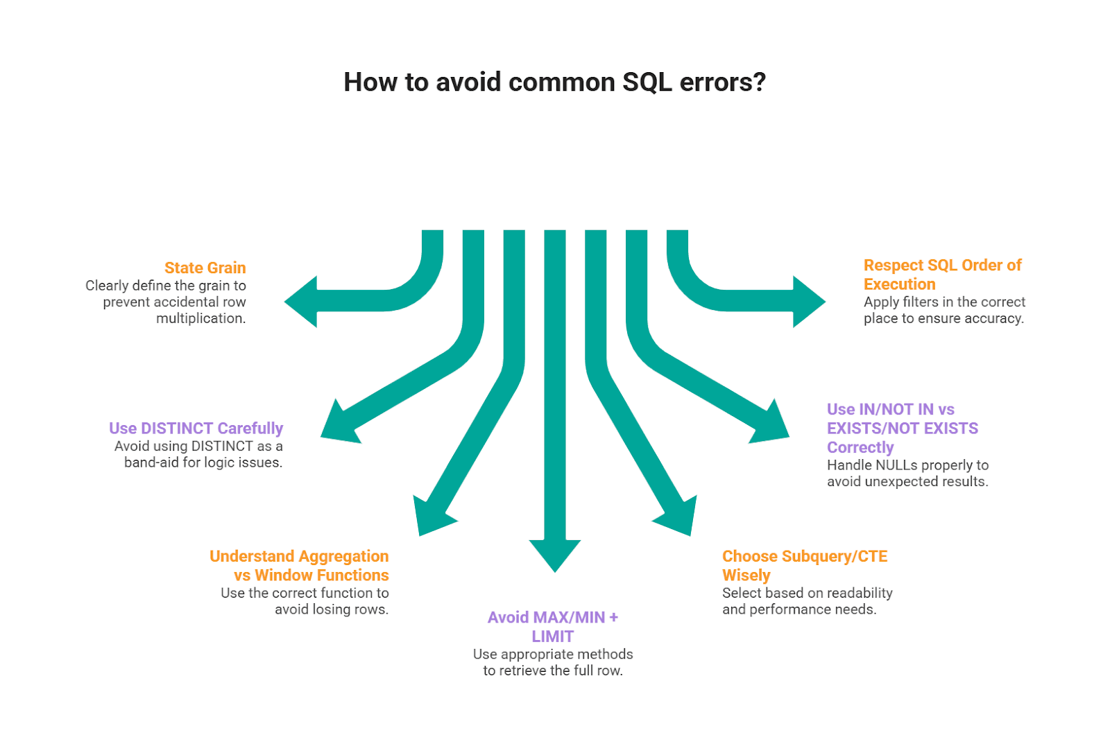
Scenario prompts are designed to surface reasoning gaps instead of syntax gaps. Here are the mistakes that show up across the patterns we used in this article.
1) Not stating the grain and accidental row multiplication
A common mistake we see candidates make is jumping into joins before they say what one output row represents.
In scenario questions, that usually leads to a silent join explosion (e.g., “one row per user” becomes “one row per user per event per day”).
If your final numbers look “too big,” this is usually why. StrataScratch’s join walkthroughs emphasize that join choice and join path change the outcome, so you want to be explicit about relationship keys and whether you’re preserving or expanding rows.
2) Using DISTINCT as a band-aid for logic issues
DISTINCT can hide problems (especially duplicate-causing joins), still pass a small test case, and then fail on real data.
It’s better to fix the root cause: correct join keys, pre-aggregate, or use a ranking window to select the intended row. This kind of “it works, but it’s fragile” solution shows up frequently in common SQL error patterns.
3) Confusing aggregation vs window functions (and losing rows)
Window functions are popular in interviews because they let you compute metrics without collapsing rows, but candidates often mix them up with GROUP BY logic or use the right function for the wrong purpose.
Pay attention to the key distinction: aggregates reduce rows; windows keep rows and add calculated values.
If you don’t leverage that correctly, you either (a) lose detail you still need later, or (b) end up re-joining to recover it.
Rule of thumb: if you need “top per group” or “rolling metric but keep row detail,” reach for windows; if you truly want one row per group, aggregate.
4) MAX/MIN + LIMIT style errors when you need the full row
Interviewers love “find the user with the max X” because it exposes a classic mistake: using MAX()/MIN() (or LIMIT 1) without guaranteeing you’re returning the correct row tied to that
Fix patterns: Rank with ROW_NUMBER() / DENSE_RANK() and filter, or join back to the aggregated result on the key + value.
5) Subquery/CTE choice without a reason (readability vs performance)
CTEs are great for interview execution because they make logic testable step by step, but they’re not automatically “better.”
We frame query structure as a balance between correctness, readability, and efficiency. Also, CTEs have real tradeoffs depending on the database and whether the engine materializes them.
6) Misusing IN/NOT IN vs EXISTS/NOT EXISTS (especially with NULLs)
Scenario questions often include “users who did X but not Y.” That’s where people reach for NOT IN and get bitten by NULL behavior, or write an IN subquery that’s less efficient than a correlated EXISTS.
Our subquery guide highlights these operators as common interview tools and also where candidates tend to get tripped up when the data isn’t clean.
7) Ignoring SQL’s order of execution and filters applied in the wrong place
Even when the syntax is valid, logic can be wrong if you filter in the wrong phase (e.g., filtering after a join that already duplicates rows, or using WHERE when you need HAVING).
SQL Dialect Notes
The solutions here use a Postgres-leaning style. If you’re interviewing in another dialect, the logic is the same, you mainly translate a few functions and a couple of patterns.
Datetime Essentials
These cover the highest-frequency interview translations: month bucketing/formatting, and date differences.
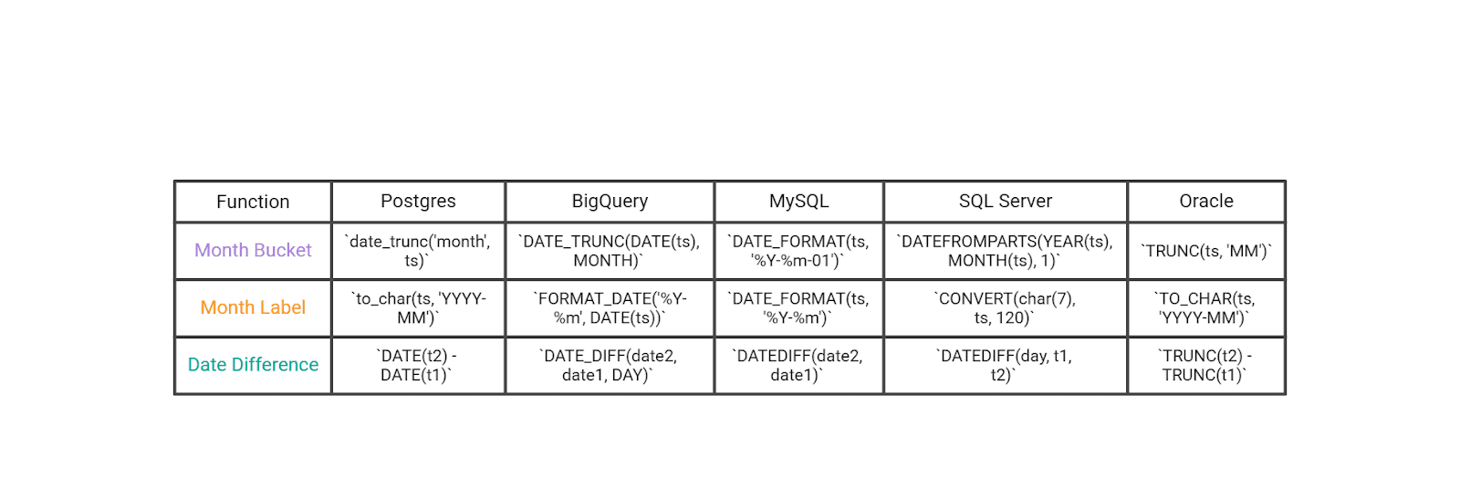
If you’re dealing with timestamps (not dates), normalize first (cast to date or truncate) before you do “per day / per month” logic.
General SQL Patterns That Show up in These Scenario Questions
These aren’t about syntax trivia, they’re the patterns interviewers actually score: cohorts, top-per-group with ties, and anti-joins.
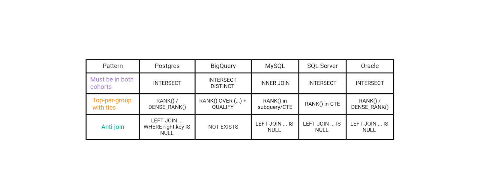
A small “seniority signal” move in interviews is to name the trade-off: INTERSECT is clean and readable when supported, but EXISTS/HAVING is often more portable across MySQL-style environments. Same logic, different constraints.
Conclusion
Scenario-based SQL questions are popular because they look like real work: you’re given a business situation, you translate it into a precise definition (grain, filters, joins, time window), and you defend why your query is correct under messy data conditions.
Across the questions in this article, the practical “interview core” repeats: you bucket and format time cleanly, compute date differences correctly, and then apply a small set of high-value patterns, cohorts (“must have both”), top-per-group with ties, and anti-joins (“include X but exclude Y”).
Datetime manipulation shows up constantly because timestamped data is everywhere, and using the right built-in functions can save you from extra subqueries and fragile logic.
Remember: you can explain your assumptions out loud, state the grain before you code, and choose patterns that are both correct and easy to validate, you’ll look much more “senior” than someone who only produces a query that runs.
Share