How To Pass Data Interviews for Machine Learning Engineer Roles

How do you get a machine learning engineer job? By passing the interviews, obviously. In this article, we deal with exactly that by detailing how to prepare.

You walk into a machine learning engineer interview, and you’ve already failed. Why? Because you think it’s all about modeling.

On the surface, they look like that. In reality, many actually test whether you can shape raw data into reliable training sets.

In this article, I’ll show you what interviewers care about most where candidates slip and how you can answer dataset questions with far more confidence.

Why ML Engineers Are Tested on Data

Because data is eve-ry-thing in ML modeling. Join data badly, label it loosely, or build it with leakage hidden inside, and you’ve got yourself a nice, shitty model. 

That’s why data interviews matter: interviewers want proof that you can turn messy production data into something a model can actually learn from.

Why do they want to see that? Spending more time shaping data than turning an algorithm is the actual description of a machine learning engineer's job. I have seen strong candidates talk beautifully about XGBoost or embeddings, then lose momentum once a panel asks how they would define a label window. 

Testing on data also reveals whether you understand business behavior. When churn gets translated into tables, you need to know what happened first, what happened later, and what shouldn’t be visible at training time.

What Interviewers Are Actually Testing

Here’s an overview of areas that are tested, which we’ll explore in more detail below. (What does a machine learning engineer do?)

In one of the following sections, I’ll show you a 30-day churn example. This is an ideal point to start angling towards it, so the points below don’t feel too general.

1. Can You Define the Prediction Problem Clearly

Getting this right is what all the subsequent steps depend on. Define the problem poorly, and even the most perfect coding skills won’t save you from getting a useless dataset. 

The interviewers especially want to see you clearly define these. 

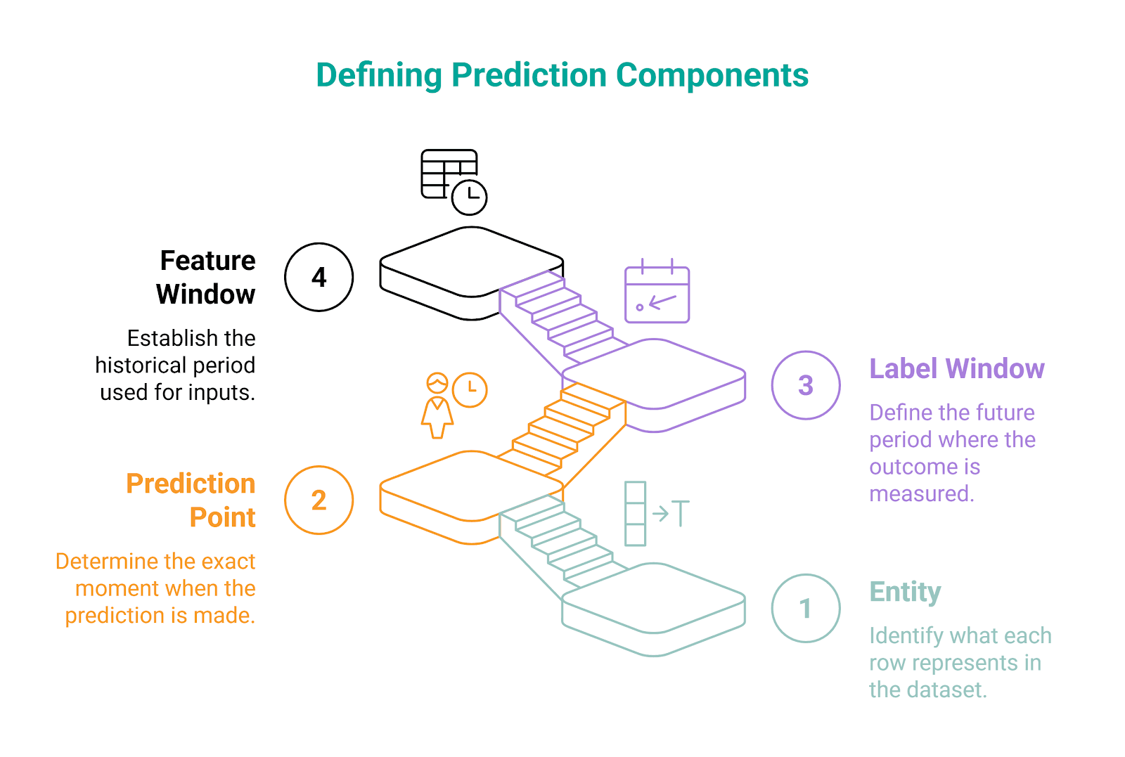
Here are examples of what these mean in practice:

• Entity: Usually a user account, device, order, or listing
• Prediction point: Could be the end of the day, the signup date, the subscription renewal date, or the first purchase date
• Label window: For example, churn within 30 days after the prediction point
• Feature window: For example, product usage in the 90 days before the prediction point

In the real interview, strong candidates would say something like this before coding:

One row will represent one active user [entity] as of January 31 [prediction point]. Features come from the prior 90 days only [feature window]. Label equals 1 if that user becomes inactive in the next 30 days [label window].  

This is an easy way to show you’re aware that you’re designing a learning problem, not just solving a joining task. Slow down, take a deep breath, and define prediction components before you jump into code. 

2. Do You Understand Time and Leakage

This is one of the biggest separators in ML engineering interviews. You can write a technically valid query and still fail because time logic breaks model realism. 

You must show that you understand one simple rule: At prediction time, you only get access to past and present data. Never future data.

To show that, you should ask questions like:

• What date are we pretending prediction happens on?
• Which events occur before that point?
• Which events define the label afterward?
• Are any features accidentally peeking into future behavior?

Why is this important? Take an example of a 30-day churn. If you have a days_since_last_login feature that uses activity that happened inside the label window, then you leaked future information. Because of that, your model performance will look amazing in testing but will probably collapse in production. You fed it future facts, not real predictive signals.

In the interview, you should proactively guard against that by saying things like:

• I’ll cap feature extraction at the prediction date.
• I’ll compute churn only after that date.
• I’ll check whether any snapshot columns were backfilled later. 

3. Can You Reason About Table Grain and Joins

Experienced machine learning engineers often follow this pattern when building the dataset. 

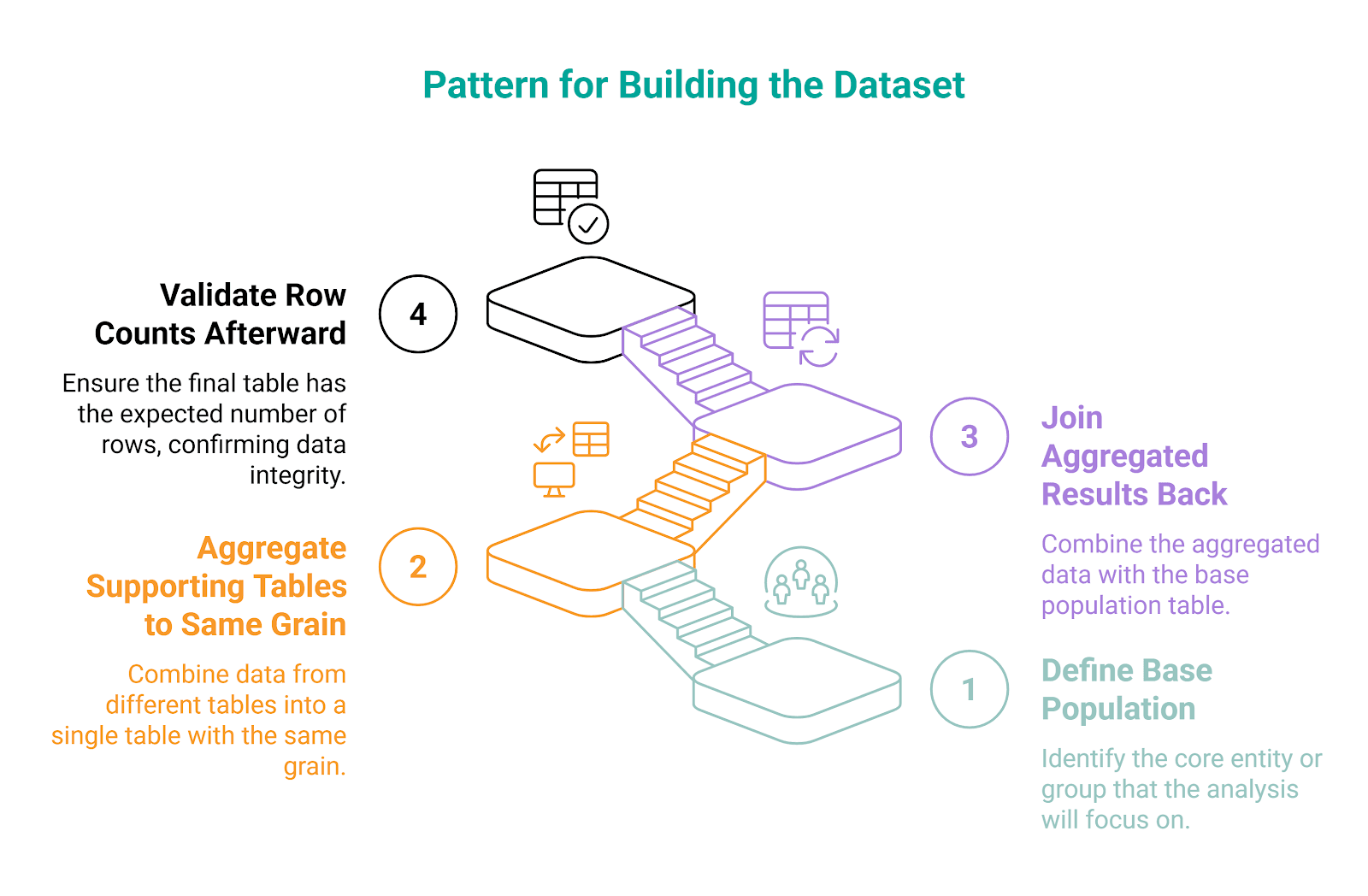
The essential concepts here are grain and joins.

Grain means what one row represents in each table. For example, it can be:

• users table: one row per user
• sessions table: one row per session
• transactions table: one row per purchase

If you’re not aware of different grains and you join the tables carelessly (one-to-many), you could duplicate rows and inflate counts. You mess up the model training with that, as the model gets trained on distorted features. 

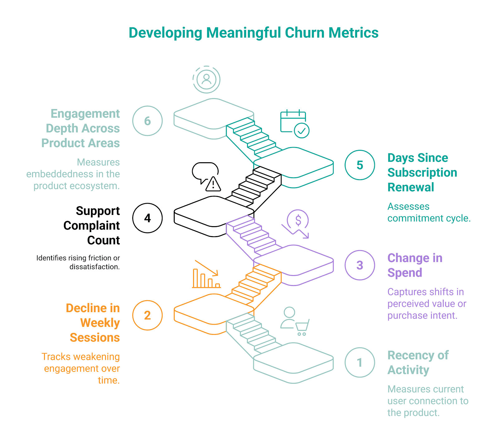
4. Can You Identify a Useful Signal Instead of Random Metrics

Not anything that can be measured belongs in a model. Interviewers want to see that you can choose features that are meaningful for the problem at hand. 

Don’t just throw everything - all the clicks, purchases, views, logins - in and hope something sticks. Think about what behavior suggests a future outcome. 

For the churn prediction model, you may choose these signals. They all capture a change in user state, not just a raw number.

5. Can You Translate Messy Business Language Into Exact Labels

In interviews, like in an actual job, the questions never arrive in clean ML notation. They will sound more like “Predict churn 30 days”, a vague business language that makes every task seem simple, when it’s far from it.

To predict churn in 30 days, you need clarifications and assumptions:

• What counts as churn
• No login for 30 days
• Subscription canceled
• No purchase for 30 days
• No core action completed
• Which users belong to the population
• All users
• Only paid users
• Only currently active users
• When does the label begin
• The day after the prediction point
• Same-day cutoff
• After the last observed activity

Using those assumptions, show judgment by saying:

I’ll define churn as having no product sessions in the next 30 days among users who were active in the prior 14 days. If business defines churn as subscription cancellation instead, I would swap label logic accordingly. 

6. Can You Explain Tradeoffs and Validate Your Own Work

ML engineering is not about finding the ideal solution. There are always tradeoffs in making decisions and choosing the right approach to a problem. 

You should be aware of assumptions, limitations, and checks. That’s why interviewers love candidates who prompt themselves on validation.

Core Data Skills ML Engineers Are Expected to Know

For machine learning engineers, both SQL and Python are essential languages. However, for data interviews, SQL is a primary language. So, when we talk about core data skills, we will focus on SQL in machine learning engineer interview questions.

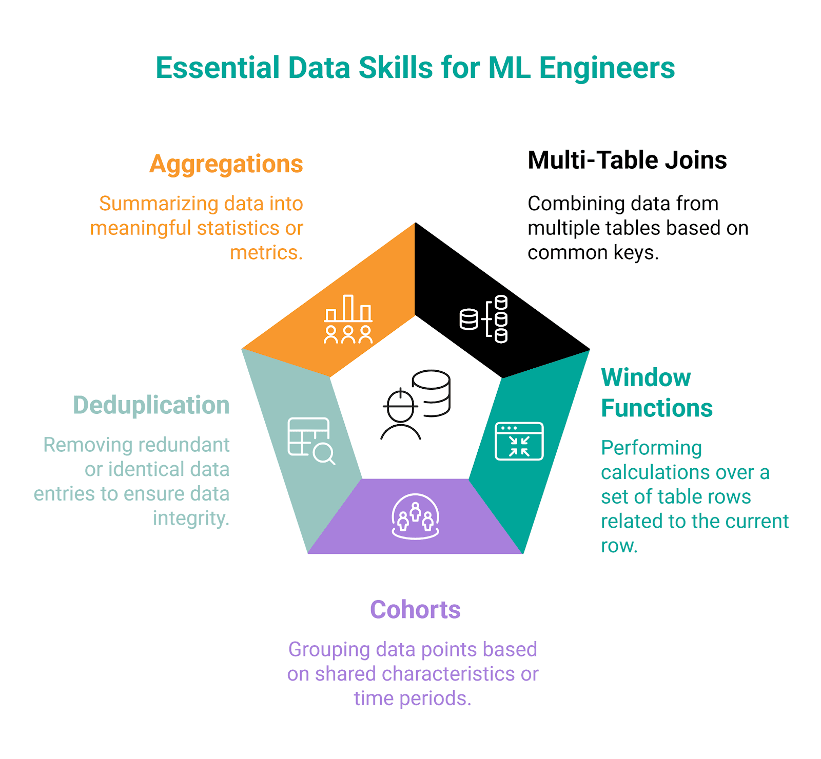
Skill #1: Multi-Table Joins

Machine learning datasets don’t live in one clean table. To be fair, they don’t typically live in two tables, either.

When you work with data, you’ll most likely have to join multiple tables when querying them. 

Syntax

If you know how to join two tables, you also know how to join three or more tables. The syntax is the same; you just keep on chaining the joins.

When joining three or more tables, JOIN or LEFT JOIN is typically used. 

SELECT t1.column_a,
       t2.column_b,
       t3.column_c
FROM table_1 AS t1
JOIN table_2 AS t2
ON t1.key_column = t2.key_column
JOIN table_3 AS t3
ON t1.key_column = t3.key_column;

Example

Here’s a question from Microsoft interviews. 

Dataset

To solve this problem, you need to join three tables. 

The first one is ms_user_dimension, which maps each user_id to an acc_id. 

The second table (ms_acc_dimension) shows whether the account is a paying customer. 

The final table is ms_download_facts, showing downloads by user_id and date.

Solution

A strong answer doesn’t just join the tables correctly. It should show your understanding of how records relate - in this case, across user, account, and activity data. In other words, you must understand the grain before joining. 

In our example, downloads are at the user-date level, while payment status is at the account level. To get the downloads for paying and non-paying users, we need to get from user_id to acc_id via the user dimension table. 

The solution logic is:

1. Joining downloads to users
2. Joining users to accounts
3. Grouping by date
4. Splitting downloads into paying and non-paying totals
5. Filtering to dates where non-paying downloads exceed paying downloads

Run the code to see the output.

Skill #2: Window Functions

In machine learning engineering work, window functions often come up because they help you keep row-level detail, while adding ordering, comparison, or aggregation. 

Here are the most commonly used functions.

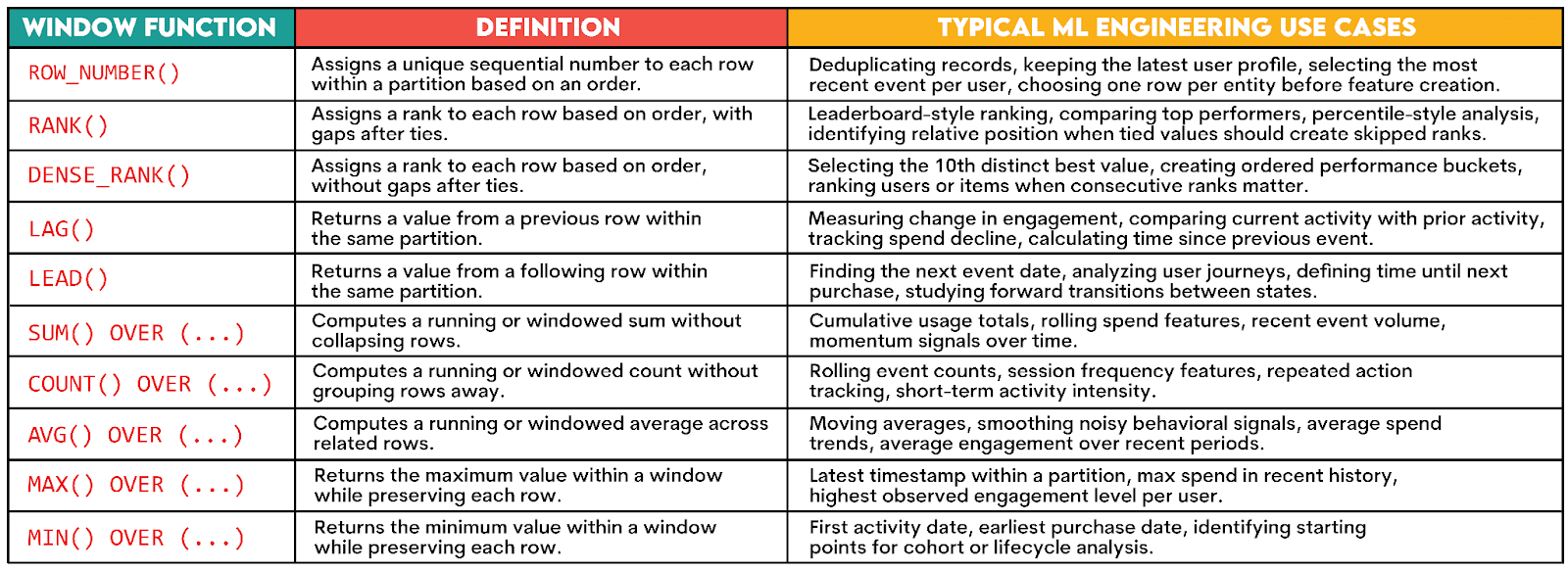
Syntax

The syntactical template for writing window functions looks like this.

SELECT column_1,
       column_2,
       function_name(expression) OVER (PARTITION BY partition_column ORDER BY order_column) AS window_result
FROM table_name;

Here’s the explanation:

• function_name(expression): The name of the window function you want to use, e.g., SUM().
• OVER (...): A mandatory clause that means the function should be treated as a window function.
• PARTITION BY partition_column: An optional clause that splits data into groups (partitions) before applying the function based on the partition_column, e.g., user_id.
• ORDER BY order_column: An optional clause (except for the ranking window functions) that sorts the rows within each partition, i.e., determines the order in which the function will be applied.

Now, let’s see how this works in practice.

Example

This question from EY and Deloitte asks you to calculate how much absolute time separates Chris Doe from the 10th-best net time (in ascending order), without gaps in ranking.

Ranking rows based on some metric is a common interview pattern. 

Dataset

There’s only one table, marathon_male.

Solution

This question tests whether you know which ranking window function to choose. It says “avoid gaps in the ranking calculation”, so that’s a signal you must use DENSE_RANK() - it doesn’t leave gaps, unlike RANK(). 

This is a three-part problem:

1. Find Chris Doe’s net_time -> the chris_doe CTE
2. Find the 10th-best runner’s time -> the tenth_runner CTE
3. Calculate the absolute difference between the times -> the final select

Skill #3: Cohorts

Cohorts help you break down data into groups based on shared characteristics. “Data”, in this case, is typically a user, customer, subscriber, etc. “A shared characteristic” could be a sign-up week, first-purchase month, or first-subscription date. 

In machine learning engineering, cohorts matter because they can mess up your labels and features. For example, a user on day 3 after signup doesn’t behave like a user on month 12. 

Cohorts are typically used to:

• Compare similar users at similar lifecycle stages
• Build retention or churn labels fairly
• Avoid mixing early users with mature users in one vague bucket

Example

To show you how cohorts are analyzed in practice, I’ll solve this Microsoft interview question. 

The question requires you to show cohort thinking because users are grouped by tenure relative to the dataset’s most recent date. 

We’ll create two lifecycle-based cohorts:

• new: registered within the last 30 days covered by the dataset (on or after 30 days before the most recent date in the dataset)
• existing: registered before new

Dataset

The dataset consists of two tables; search_events is the first one. 

The second table is accounts.

Solution

The solution is complex, but we’ll split it into six CTEs to make it more readable. 

The max_date CTE uses MAX() to find the most recent event date in the dataset. This will be a reference point for splitting users into cohorts.

WITH max_date AS
    (SELECT MAX(event_timestamp) AS max_event_date
     FROM search_events),

In user_segments, I use CASE WHEN to label each user as new or existing, depending on the registration date. I used CROSS JOIN so that each row’s (user’s) registration_date is compared to the most recent event date.

user_segments AS
    (SELECT a.user_id,
            CASE WHEN a.registration_date >= md.max_event_date - INTERVAL '30 days' THEN 'new' ELSE 'existing' END AS user_segment
     FROM accounts a
     CROSS JOIN max_date md),

The next CTE is searches. It isolates only search events.

searches AS
    (SELECT user_id,
            query,
            session_id,
            event_timestamp AS search_timestamp
     FROM search_events
     WHERE event_type = 'search'),

In the clicks CTE, I isolate click events and use ROW_NUMBER() to rank clicks within the user_id + query + session_id partition. The earliest click gets click_rank = 1 because the partition is sorted by timestamp in ascending order. 

(SELECT user_id,
            query,
            session_id,
            event_timestamp AS click_timestamp,
            ROW_NUMBER() OVER (PARTITION BY user_id, query, session_id
                               ORDER BY event_timestamp) AS click_rank
     FROM search_events
     WHERE event_type = 'click'),

The search_with_clicks CTE joins the searches and clicks CTEs and retains only the clicks ranked 1 that occurred at or after the search. It also uses EXTRACT (EPOCH…) to calculate how many seconds passed between the search and that first click. 

search_with_clicks AS
    (SELECT s.user_id,
            s.query,
            s.session_id,
            s.search_timestamp,
            c.click_timestamp,
            EXTRACT(EPOCH
                    FROM (c.click_timestamp - s.search_timestamp)) AS time_diff_seconds
     FROM searches s
     LEFT JOIN clicks c ON s.user_id = c.user_id
     AND s.query = c.query
     AND s.session_id = c.session_id
     AND c.click_rank = 1
     AND c.click_timestamp >= s.search_timestamp),

The final CTE is search_success. It joins search_with_clicks and user_segments CTEs, groups the data by the user segment, then counts total searches and successful searches using COUNT(*) and SUM(CASE WHEN…), respectively.

search_success AS
    (SELECT us.user_segment,
            COUNT(*) AS total_searches,
            SUM(CASE WHEN swc.time_diff_seconds IS NOT NULL
                         AND swc.time_diff_seconds <= 30 THEN 1 ELSE 0 END) AS successful_searches
     FROM search_with_clicks swc
     INNER JOIN user_segments us ON swc.user_id = us.user_id
     GROUP BY us.user_segment)

Now, we only need one simple SELECT that lists the required columns and calculates the success rate by dividing successful searches by total searches. 

SELECT user_segment,
       total_searches,
       successful_searches,
       successful_searches::NUMERIC / total_searches AS success_rate
FROM search_success;

Here’s the whole code.

Skill #4: Deduplication

Real-world datasets often contain duplicate records, whether by mistake or because of the data schema. 

Deduplicating such data is important for machine learning engineers because duplicate data can distort labels and inflate features, which damages your training data and, ultimately, the model’s performance. 

Common cases of duplicate data are:

• Multiple profile records per user
• Repeated payment attempts
• Several status updates for one order
• Duplicated events from tracking pipelines

SQL Pattern

The simplest way to deduplicate data is to use DISTINCT. In PostgreSQL, you can also use DISTINCT ON for keeping one row per group based on a chosen sort order. 

However, when deduplication requires keeping one row per business key, the most common and most flexible pattern uses ROW_NUMBER.

The common pattern first uses a window function, typically ROW_NUMBER(), to assign a row number within a group.

ROW_NUMBER() OVER (PARTITION BY column_1 ORDER BY column_2 [ASC] [DESC]);

Here, PARTITION BY defines the duplicate group, and ORDER BY decides which row gets ranked first and in which order (ascending or descending).

RANK() and DENSE_RANK() are used less commonly because ties can create multiple rows.

The ranking part of the pattern is then followed by filtering. 

WHERE row_number = 1

Example

I’ll show you how to deduplicate data by solving this Redfin interview question.

Dataset

The dataset consists of the table redfin_call_tracking. 

Solution

To solve this problem, we need to identify the first call per request and treat every subsequent call as an update call. This is a deduplication problem because we will separate one special row from the rest within each request_id group. 

First, there’s a SELECT statement with ROW_NUMBER() which ranks calls in ascending order (from the oldest to the newest) for each request_id.

SELECT *,
       ROW_NUMBER() OVER (PARTITION BY request_id ORDER BY created_on) AS rk
        FROM redfin_call_tracking

In the next step, the above statement becomes a subquery in a SELECT that returns only the IDs of calls that are not the first call.  

SELECT id
     FROM
       (SELECT *,
               ROW_NUMBER() OVER (PARTITION BY request_id ORDER BY created_on) AS rk
        FROM redfin_call_tracking

The final step is to turn all the above code into a subquery in the main SELECT that calculates the average call duration. 

Here’s the whole code. 

Skill #5: Aggregations

Knowing how to aggregate data is an important skill because raw event tables seldom become model-ready features on their own. 

Typical aggregation that machine learning engineers perform is aggregating behavior over a time window, e.g.:

• Count actions
• Sum spend
• Measure recency
• Compute averages
• Compare short and long windows

Let’s demonstrate this in an actual interview question.

Example

This is a classic aggregation problem because we need to summarize workers by department and count how many joined on or after April 1, 2014. 

Data

We’ll use the worker table.

Solution

In the solution, I first filter data in a CTE to keep only the workers who joined on or after 2014-04-01.

WITH filtered_worker AS (
  SELECT *
  FROM worker
  WHERE joining_date >= DATE '2014-04-01'
)

In the final step, SELECT calculates how many workers belong to each department. 

Interview-Style Example: Build a Labeled Dataset (Churn in 30 Days)

We’ll now take this talk about data and SQL concepts to another level.

A common interview pattern is for the interviewer to test whether you can turn raw user activity into a training table.

The Setup

Predicting churn, the percentage of users who leave, is a common model that machine learning engineers work on, so many interviews focus on it. Our example will, too.

Assume the interviewer asks: “Build a dataset for predicting whether a user will churn in the next 30 days.”

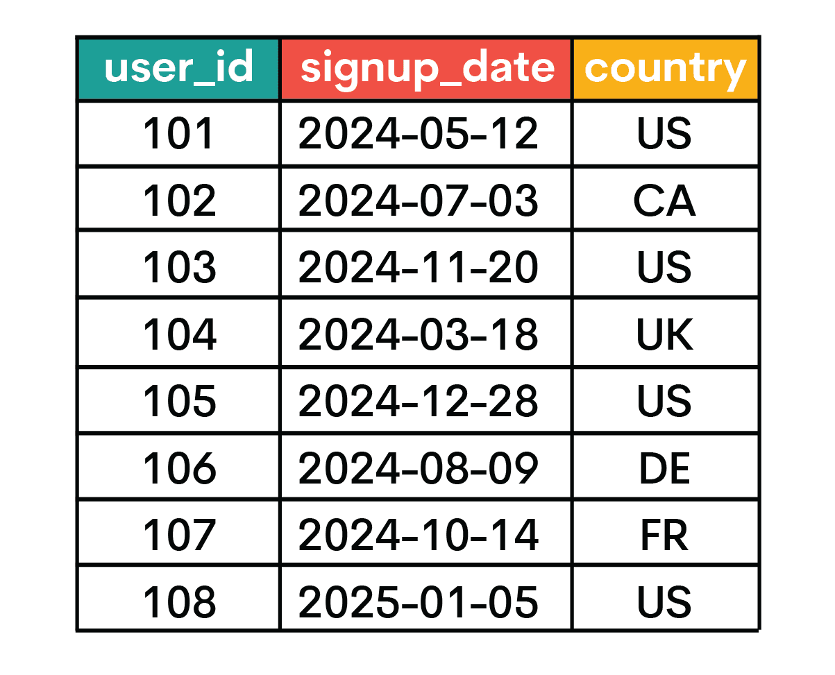
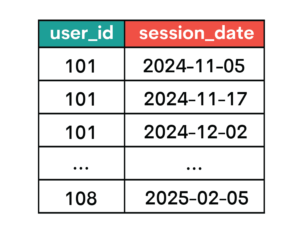
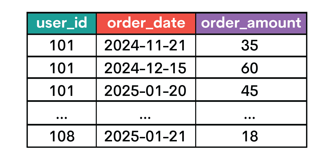
Data

They then give you this raw data to work with. 

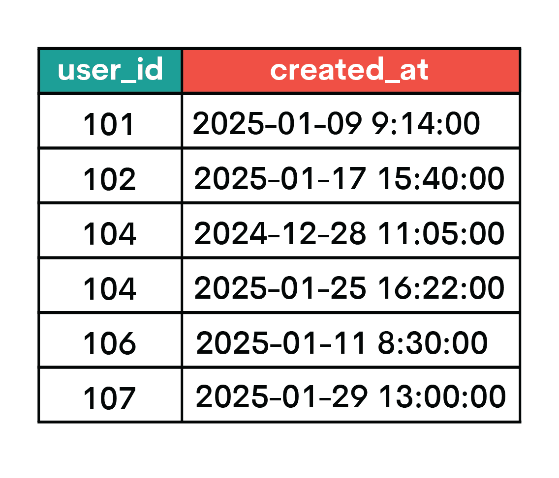
The first table is named users.

The second is sessions.

You also have the orders table. 

The final table is support_tickets.

Run this script to create the dataset locally.

Now, the steps you need to follow in the interview.

Step #1: Assumptions

First, you have to state the assumptions you’ll work with.

• Entity: one row per user
• Prediction date: 2025-01-31
• Feature window: 2024-11-02 to 2025-01-31
• Label window: 2025-02-01 to 2025-03-02
• Churn definition: a user is churned if they have no session activity during the label window

Step #2: Explaining the General Approach

Next, you briefly explain the concept, for example, like this. 

To build a labeled churn dataset, I’ll first choose the prediction date: 2025-01-31 in this case. Then, I will summarize past user behavior into features. After that, I will look forward into the label window and mark whether each user churned.

The rule is always the same: past data is features, future data is labels. 

Step #3: Explaining the Coding Logic

Before you write the SQL code and build an actual dataset, explain the coding sequence.

1. Defining the base population
2. Building session, order, and support features from the 90-day feature window
3. Finding which users were active in the next 30 days
4. Assigning the churn label
5. Joining everything into one row per user

Step #4: SQL Coding

Here’s the code you should write to build the dataset. 

WITH base_users AS (
    SELECT
        user_id
    FROM users
    WHERE signup_date <= DATE '2025-01-31'
),

session_features AS (
    SELECT
        user_id,
        COUNT(*) AS sessions_90d,
        COUNT(DISTINCT session_date) AS active_days_90d,
        MAX(session_date) AS last_session_date
    FROM sessions
    WHERE session_date >= DATE '2024-11-02'
      AND session_date <= DATE '2025-01-31'
    GROUP BY user_id
),

order_features AS (
    SELECT
        user_id,
        COUNT(*) AS orders_90d,
        SUM(order_amount) AS spend_90d,
        AVG(order_amount) AS avg_order_value_90d
    FROM orders
    WHERE order_date >= DATE '2024-11-02'
      AND order_date <= DATE '2025-01-31'
    GROUP BY user_id
),

ticket_features AS (
    SELECT
        user_id,
        COUNT(*) AS tickets_90d
    FROM support_tickets
    WHERE created_at >= TIMESTAMP '2024-11-02 00:00:00'
      AND created_at < TIMESTAMP '2025-02-01 00:00:00'
    GROUP BY user_id
),

future_activity AS (
    SELECT DISTINCT
        user_id
    FROM sessions
    WHERE session_date >= DATE '2025-02-01'
      AND session_date <= DATE '2025-03-02'
),

labels AS (
    SELECT
        b.user_id,
        CASE
            WHEN f.user_id IS NULL THEN 1
            ELSE 0
        END AS churn_30d
    FROM base_users b
    LEFT JOIN future_activity f
        ON b.user_id = f.user_id
)

SELECT
    b.user_id,
    COALESCE(s.sessions_90d, 0) AS sessions_90d,
    COALESCE(s.active_days_90d, 0) AS active_days_90d,
    s.last_session_date,
    COALESCE(o.orders_90d, 0) AS orders_90d,
    COALESCE(o.spend_90d, 0) AS spend_90d,
    COALESCE(o.avg_order_value_90d, 0) AS avg_order_value_90d,
    COALESCE(t.tickets_90d, 0) AS tickets_90d,
    l.churn_30d
FROM base_users b
LEFT JOIN session_features s
    ON b.user_id = s.user_id
LEFT JOIN order_features o
    ON b.user_id = o.user_id
LEFT JOIN ticket_features t
    ON b.user_id = t.user_id
LEFT JOIN labels l
    ON b.user_id = l.user_id
ORDER BY b.user_id;

Step #5: Interpreting the Code

You should now explain what you did in the code to show you didn’t just memorize the solution.

There are six CTEs in the code. The first one is base_users, which defines who belongs in the dataset, which are users who signed up on or before 2025-01-31, the prediction date. 

The second CTE (session_features) selects the users with sessions between 2024-11-02 and 2025-01-31, a 90-day feature window. It then calculates the session count, the number of active days, and the latest session date for each user.

Next, we have order_features. It selects the users with orders in the same 90-day feature window as earlier. We count those orders, then sum their amounts and calculate the average value per user.  

The ticket_features CTE counts support contrast during the same historical window. 

In future_activity, we select unique users with at least one session in the next 30 days, i.e., within the label window, defined as 2025-02-01 to 2025-03-02. This CTE supports label creation in the last CTE.

We do that by performing a LEFT JOIN on the base_users and future_activity CTEs, then using CASE WHEN to assign the 1 label to users that don’t appear in future_activity, i.e., they churned in 30 days. 

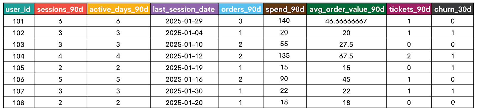
The final SELECT statement joins all feature tables and the label table to the base users, which creates the dataset shown below. 

Step #6: Why the Features Matter

You have to explain why you chose specific features and why they matter. This will show you understand what you’re doing, and it’s an additional check for you to confirm you got all the features. 

In our example, each feature was chosen because it captures a different part of user behavior that can change before churn happens.

• sessions_90d: Measures overall engagement volume, as users with fewer sessions over 90 days will probably be less engaged, therefore more likely to leave. 
• active_days_90d: Captures engagement consistency, not just volume. For example, if two users have the same number of sessions, the healthier behavior is for those sessions to be spread across more days. 
• last_session_date: This feature reflects recency, as users with recent sessions are less likely to churn than those who haven't had a session in a long time. 
• orders_90d: Measures commercial activity. If a user stops purchasing, that probably means the product's value has decreased for the user. 
• spend_90d: This is to show the total value dimension. A drop in spending often reflects a change in commitment, not just a lower count of transactions.
• avg_order_value_90d: This feature helps in distinguishing between users who spend often but less and those whose purchases are seldom but spend more. 
• tickets_90d: With this feature, we capture friction, as support activity can signal dissatisfaction with the product and the increased probability of churn.

Step #7: Dataset Validation

Once you have the dataset, Python steps in instead of SQL. Python is typically used for:

• Dataset inspection
• Feature validation
• Model training
• Preprocessing
• Experimentation

We won’t go any further than dataset inspection; this is where the scope of our article ends. 

So, when validating the dataset, you should check:

• row count - to confirm the dataset has the expected one-row-per-user structure
• label balance - to confirm the dataset has the expected one-row-per-user structure
• missing values - to catch broken joins or incomplete feature generation
• feature ranges - to make sure the values look realistic and nothing appears obviously off. 

Only mentioning this in the interview will get you points, let alone writing this code. 

import pandas as pd

# Load the labeled dataset from your computer
df = pd.read_csv("path/to/your/labeled_dataset.csv")

print(df.shape)
print(df["churn_30d"].value_counts())
print(df["churn_30d"].mean())

print(df.isnull().mean().sort_values(ascending=False))
print(df[["sessions_90d", "orders_90d", "spend_90d", "tickets_90d"]].describe())

Here’s the output.

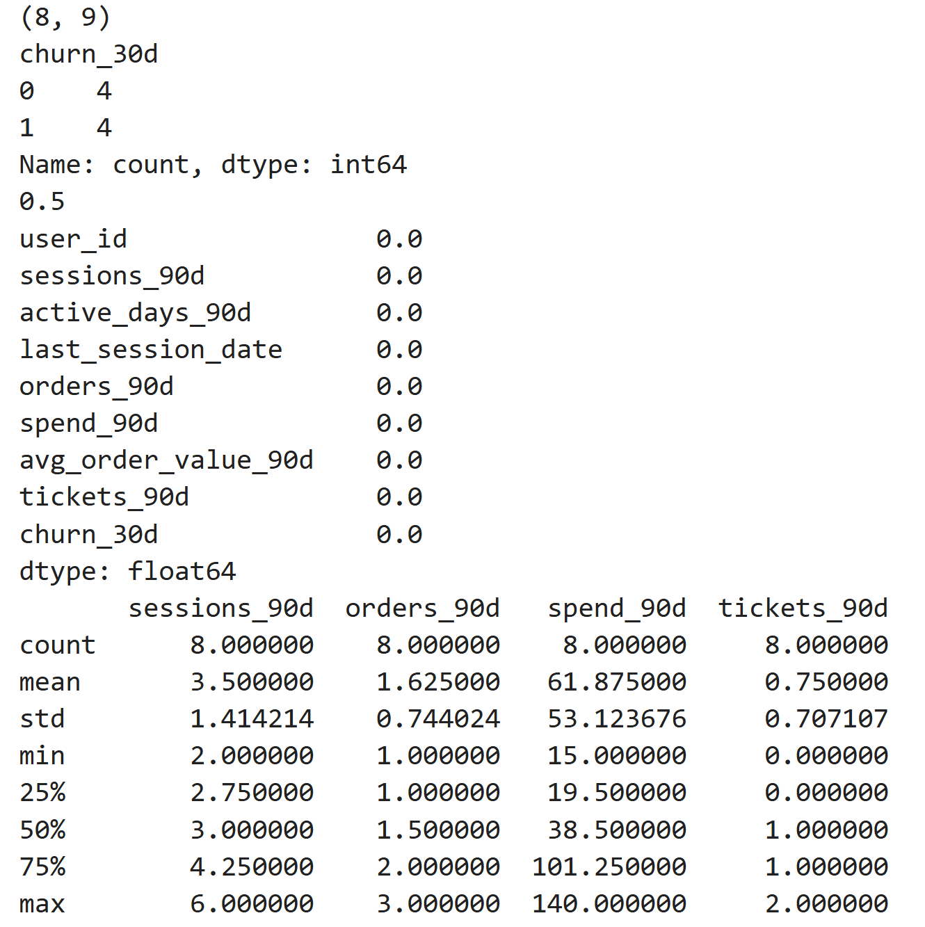
It shows that the final table has a one-row-per-user structure, as expected. There are no missing feature values, and the label distribution is balanced (there are 4 no-churn and 4 churn users). The features have sensible ranges, and nothing looks obviously broken. 

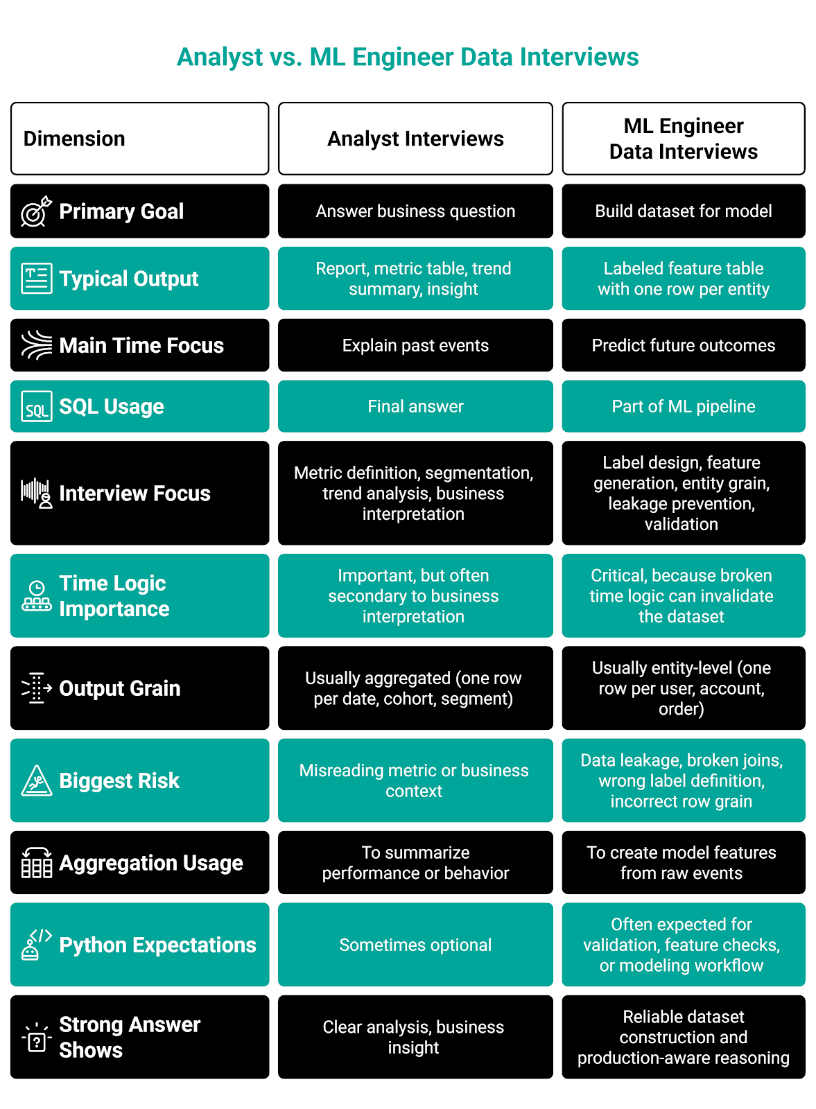
How ML Engineer Data Interviews Differ From Analyst Interviews

They might look similar because both heavily use SQL, event tables, joins, and business questions. 

In an analyst interview, you typically have to answer a reporting or decision-making question. (Think the questions I showed you in the “Core Data Skills ML Engineers Are Expected to Know” section.)

In the machine learning engineer interviews, the main goal is often to build model-ready data. 

Here’s an overview presenting the main differences. 

Common Mistakes Candidates Make in ML Data Interviews

Most candidates don’t fail the interview because they don’t know SQL. They fail because they solve the wrong problem, don’t define data precisely, or don’t think about how it would behave in production. 

Here’s an overview of those common mistakes. I’ll go into more detail below. 

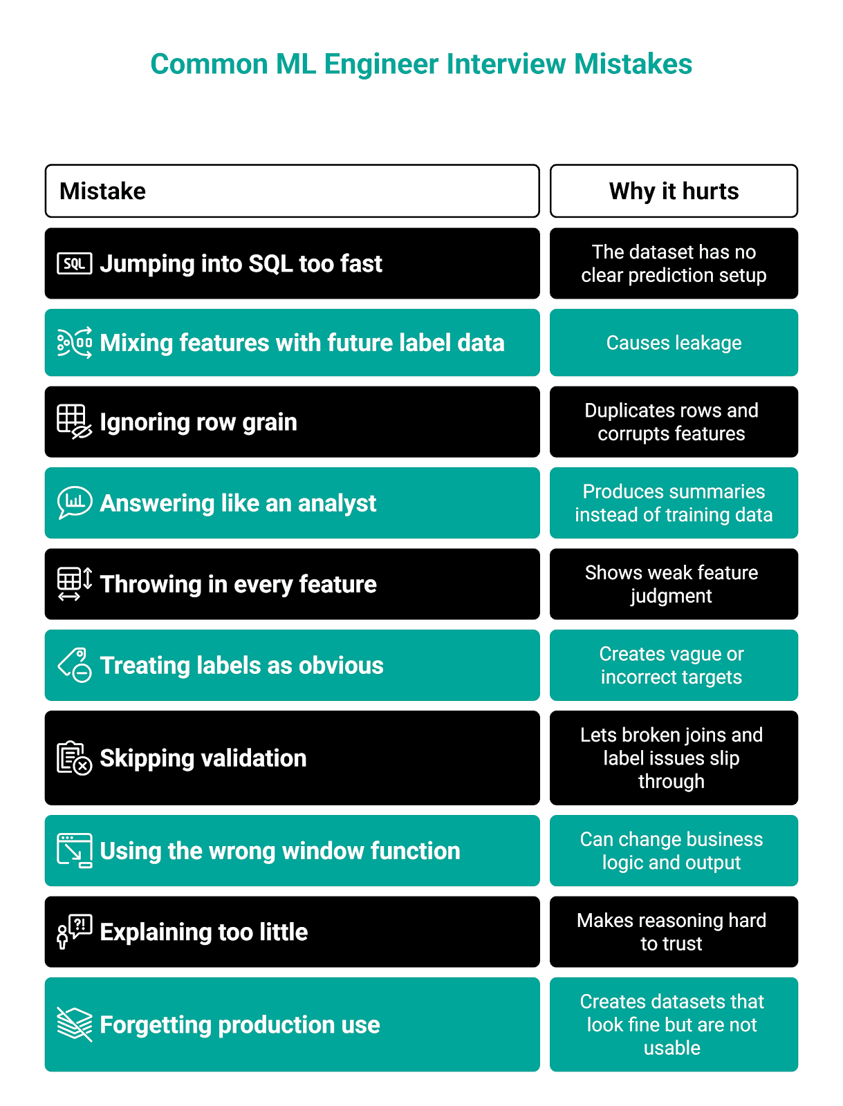
Mistake #1: Jumping Into SQL Before Defining the Prediction Setup

This one will leave a very bad impression. You can’t just start writing SQL code without defining what one row represents, when prediction happens, what the feature window is, and how the label is defined. 

A good example of how it’s done is in the “Interview-Style Example: Build a Labeled Dataset (Churn in 30 Days)” section, step one. 

Mistake #2: Mixing Feature Data With Label-Period Data

One reason for trying not to make the first mistake is that it will otherwise very easily lead to the next one: data leakage. You simply mustn’t write a query that allows the model to use future information.

This typically happens when you are:

• Using activity from the churn window inside features
• Using a status field updated after the outcome happened
• Computing recency with dates that go beyond the prediction cutoff

Mistake #3: Ignoring Row Grain

If your grain is one row per user, it should be kept in the final result, too. You always have to think about whether you need to aggregate and whether the join will duplicate rows. 

Mistake #4: Writing Valid SQL That Does Not Answer the ML Version of the Problem

Some candidates answer a machine learning interview question as if they were analysts. 

To use our churn example, the mistake would mean not building a churn dataset but outputting:

• Churn rate by month
• Average sessions by user segment
• A summary table of activity by country

Those queries might work smoothly, but that’s not what the interviewer asked of you. 

Mistake #5: Choosing Features Without Explaining Why They Matter

You shouldn’t just throw in the available metrics. You should choose those that matter and explain why they matter.

For example, see how I did it in “Interview-Style Example: Build a Labeled Dataset (Churn in 30 Days)” section, step six. 

Mistake #6: Treating Label Definition as Obvious

The interview questions often sound clear. But they’re not. They’re intentionally vague to reflect the actual prompt you’ll get from your boss at the actual job.

For example, when the interviewer asks you to predict churn in 30 days, they do so to see if you’ll state an assumption clearly. Churn could mean:

• No login
• No purchase
• Canceled subscription
• No core action completed

Interviewers know the churn definition is not universal. They want to see if you know, too. 

Mistake #7: Forgetting Validation

Most candidates will consider their answer complete once they finish the SQL code. 

Strong candidates will go one step further and explain how they would validate the dataset, which is exactly what we did in the interview-style example section, step #7. 

Even stronger candidates would write Python validation code, as we did, if asked. 

Mistake #8: Using the Wrong Window Function for the Job

Candidates often choose the ranking window function wrongly: RANK()/DENSE_RANK() when they need exactly one row, or ROW_NUMBER() when they should keep ties. 

The wrong choice may significantly alter the final output.

Mistake #9: Over-Focusing on Syntax and Under-Explaining Decisions

You might think that the best decision is to write your code in silence, so you can focus better and produce smoothly running, syntax-perfect SQL code. Wrong! 

You should explain what you do as you go. This has two benefits. First, you’ll help the interviewer understand what you’re doing and that it’s deliberate, not accidental. Second, you’ll help yourself understand what you’re doing and, potentially, catch your own mistakes and correct them before it’s too late.

Even if the code is not perfect, clear reasoning will still make your answer strong. So, explain:

• Why is this the base table
• Why a table is or is not aggregated before the join
• Why LEFT JOIN and not JOIN
• Why does the label start after the prediction date
• Why you’ll use a certain feature  

Mistake #10: Forgetting That the Dataset Has to Be Usable Later

The ML dataset that you produce doesn’t exist on its own; it’ll end up in production. In interviews, you must show you’re aware of that.

You do that by producing a dataset that:

• Does not include duplicate rows
• Does not include columns with unclear names
• Does not mix raw events with aggregates inconsistently
• Does not produce data leakage

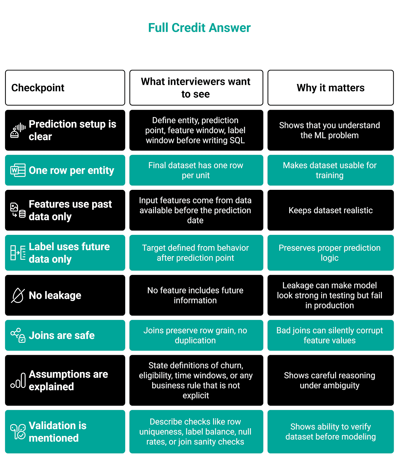
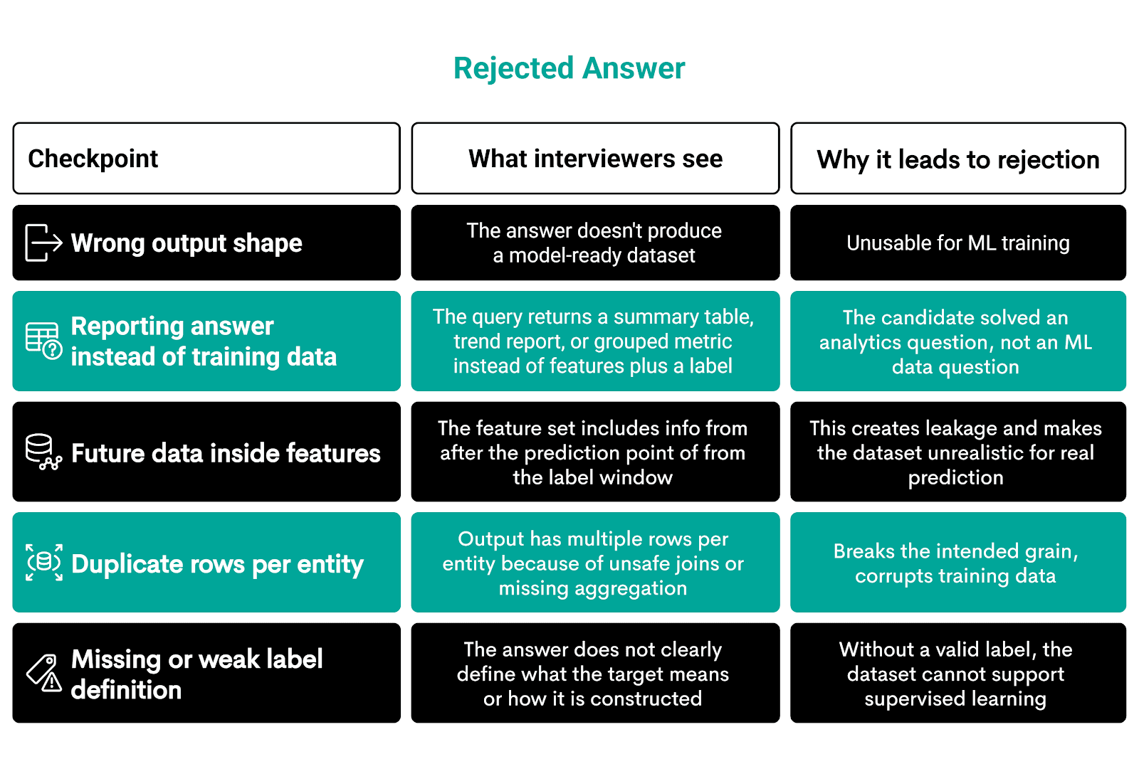
How Interviewers Evaluate Data Answers (Full vs Partial vs Reject)

If you write flawless SQL code, it doesn’t necessarily mean you’ve passed the interview. The same way, it doesn’t mean you’ll fail if your answer is imperfect.

Interviewers will grade different aspects of your answers. Let’s see what will get you full credit, what will get you a partial one, and what will get you rejected. 

Full Credit

A full-credit answer solves the right problem in the right shape. The SQL code doesn’t have to be perfect to the smallest detail, but it must show the correct general logic, which is communicated clearly. 

Here’s the evaluation checklist.

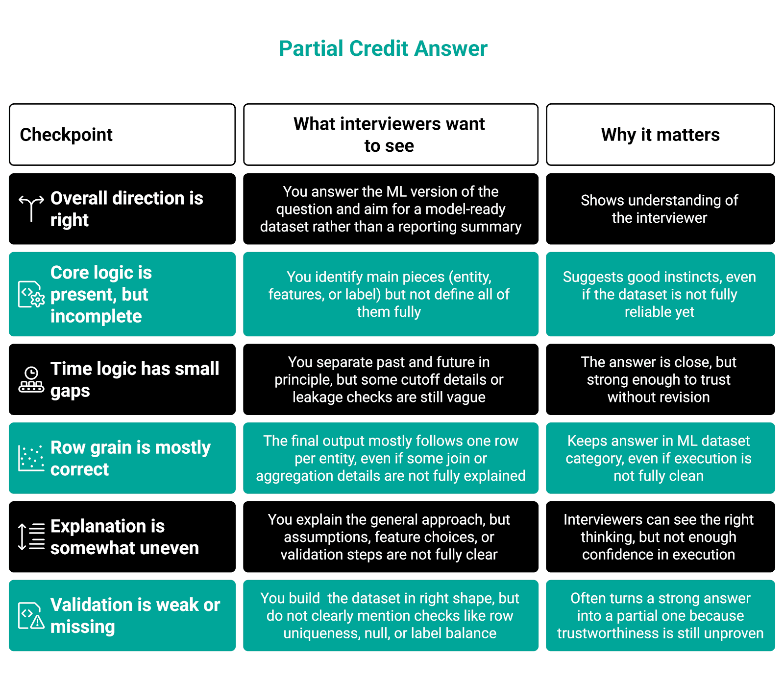
Partial Credit

This is very common. Interviewers often give partial credit when the candidate has the right general direction, but a piece or two is missing, unclear, or flawed.

Here’s the list of things that will get you partial credit. 

Rejected

Your answers will be rejected if they are fundamentally non-usable for machine learning or completely miss the interview prompt. 

One of the examples I gave earlier is that instead of building a dataset for a churn model, you simply output the churn ratio. 

Here’s what will get you rejected. 

How to Prepare Effectively (Practice Path + StrataScratch Problems)

To prepare well for the machine learning engineer interview, you need to dedicate a great deal of time to it. But you also need to prepare smartly, which means keeping your focus on the concepts tested in the actual interviews.

I would divide the preparation into three stages.

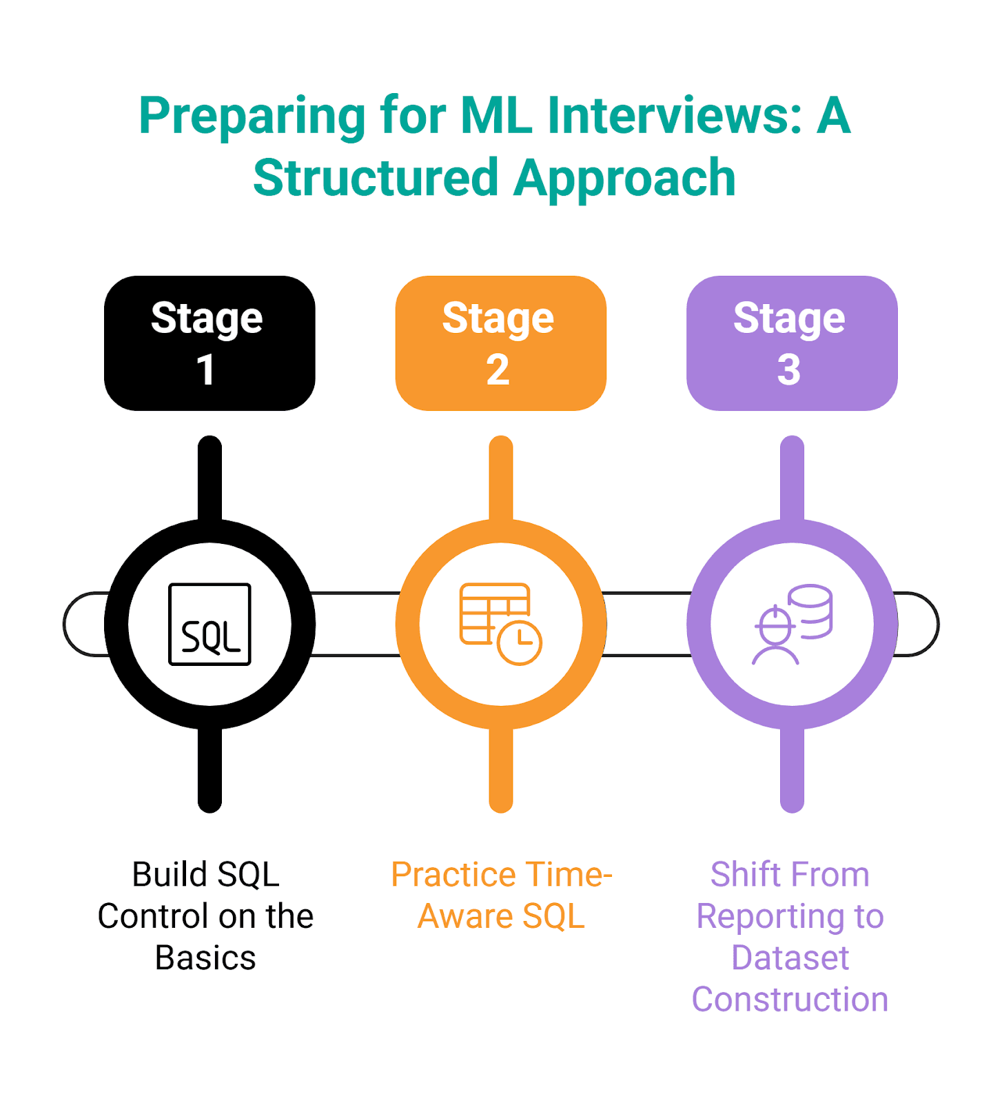
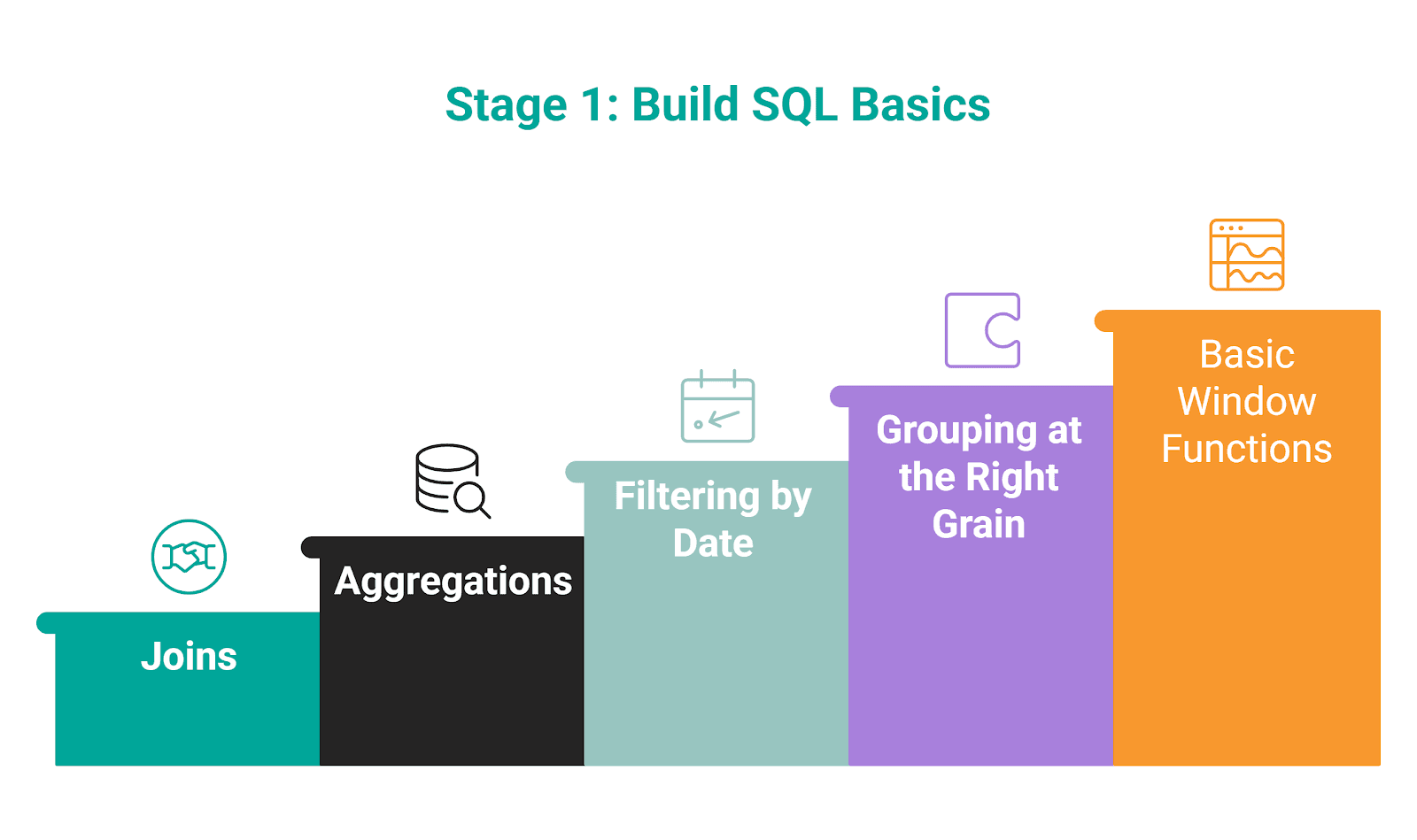
Stage 1: Build SQL Control on the Basics

You should start by building fluency in SQL basics, which are commonly used in machine learning work.

Suggested StrataScratch Problems for Practice

Here are several selected problems. These are just to get you started. Feel free to dig deeper into our question database. 

Question #1: Find All Posts Which Were Reacted to With a Heart

Try to solve it here.

Question #2: User Flag Performance Analysis

Try to solve it here.

Question #3: Acceptance Rate By Date

Try to solve it here.

Question #4: Income By Title and Gender

Try to solve it here.

Question #5: Highest Cost Orders

Try to solve it here.

Question #6: Proportion Of Total Spend

Try to solve it here.

Question #7: Number of Comments Per User in 30 days before 2020-02-10

Try to solve it here.

Question #8: Find the Genre of the Person With the Most Number of Oscar Winnings

Try to solve it here.

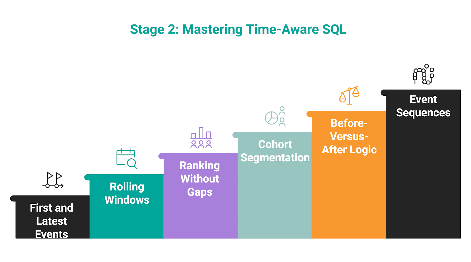
Stage 2: Practice Time-Aware SQL

Once you’ve established the basics, the next important step is to focus on time logic in SQL. This will get you ready to build realistic features from data, which is also the next step in interview preparation.

Suggested StrataScratch Problems for Practice

Here are several selected problems I’d recommend that you solve.

Question #9: Revenue Over Time

Try to solve it here.

Question #10: Player with Longest Streak

Try to solve it here.

Question #11: Top Actor Ratings by Genre

Try to solve it here.

Question #12: Monthly Percentage Difference

Try to solve it here.

Question #13: Customer Tracking

Try to solve it here.

Question #14: Product Engagement Momentum Shifts

Try to solve it here.

Question #15: Top Sunny Locations By Hours

Try to solve it here.

Question #16: Five-Year Sales Growth Regions

Try to solve it here.

Question #17: Top Customers With Dense Ranking

Try to solve it here.

Question #18: Lowest Priced Orders

Try to solve it here.

Question #19: Monthly Sales Rolling Average

Try to solve it here.

Question #20: Finding User Purchases

Try to solve it here.

Question #21: Premium Accounts

Try to solve it here.

Stage 3: Shift From Reporting to Dataset Construction & Model Building

This is the crucial stage that most candidates omit from their interview preparation. To pass data interviews for machine learning engineer roles, you’ll need to make that extra push to stand out from the crowd: practice dataset construction.

I showed you earlier how to do that. Knowing how to construct ML datasets is essential for machine learning engineers, as that’s what you’ll do in the actual job. Practicing that skill shifts you from analyst-style problems (the first two preparation steps, where the goal is to explain what happened) to honing the ML engineer mindset of building data that can predict what happens next, i.e., building the machine learning model.

The best way to practice this skill is to do machine learning projects.

Suggested StrataScratch Projects for Practice

Here are several projects I selected for your practice. 

Project #1: Delivery Duration Prediction

DoorDash: Predict order arrival times using stacked regression with prep-time decomposition. Python, LGBM, Scikit-learn, Keras.

Project #2: Prediction of Stock Price Direction

NeuroTrade: Forecast stock price direction using ensemble classifiers and trend features. Python, Scikit-learn, TensorFlow, Pandas.

Project #3: Fraudsters Detection

This data project has been used as a take-home assignment in the recruitment process for the data science positions at Revolut.

Project #4: Predicting Price

Haensel AMS: Optimize price prediction via model shootout and scaler comparison. Python, Scikit-learn, LGBM, Keras.

Project #5: Customer Churn Prediction

Sony Research: Predict telecom churn via multi-model benchmarking and drift-aware deployment. Python, Scikit-learn, XGBoost, Keras.

Project #6: Driver Lifetime Value

Lyft: Segment drivers by lifetime value using K-Means clustering and retention analysis. Python, Pandas, Scikit-learn, Seaborn.

Project #7: Response to Marketing Campaign

SparkCognition: Optimize campaign targeting via LightGBM with native categorical encoding. Python, LightGBM, Scikit-learn, Pandas.

Project #8: Property Click Prediction

NoBroker: Forecast property interactions using multi-model regression and corrupted JSON recovery. Python, Scikit-learn, XGBoost, Keras.

Project #9: U.S. Occupational Wage Analysis

BLS: Decode U.S. wage inequality using hypothesis testing and regression analysis. Python, Scipy, Statsmodels, Matplotlib.

Project #10: Modelling Churn in Energy Company

BCG Gamma: Exploring SME energy customer churn data and 2015 pricing to uncover patterns, insights, and key questions.

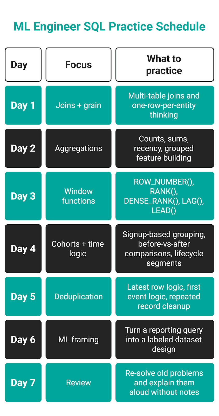
Weekly Practice Path

Over the course of one week, I would create the path like this. 

Conclusion

With this article, you’re equipped for success at machine learning engineer interviews. 

We covered core skills you need to hone, interview-style examples, common mistakes at interviews, and how interviewers evaluate answers. Finally, there’s a very useful section with many real interview questions you can use for preparation. 

Frequently Asked Questions

1. What do ML engineers get tested on in SQL interviews?

The core area you will get tested in is building datasets from row tables. This includes testing your SQL knowledge: joins, aggregations, window functions, deduplication, cohort logic, label construction, feature windows, and leakage prevention. 

If the interviewers want to test a specific SQL concept, they’ll also give an analysis question or two to solve. 

2. How do you avoid data leakage in an interview dataset question?

You avoid leakage by ensuring that features use only information available at the prediction point, i.e., you don’t use the future events to train the prediction. In practice, this means you have to define a feature window and a separate future label window. 

In addition, you should check whether status fields are updated after the outcome happened or aggregates were built with future events.

3. What’s the difference between labels and features?

Features are the input variables the model uses to make predictions, i.e., session count, total spend, or days since last login. They come from the past and present. 

Labels are the outcomes the model aims to predict, e.g., 30-day churn, fraud, or conversion. 

4. What window functions are most common in ML data interviews?

The most common are:

• ROW_NUMBER()
• RANK()
• DENSE_RANK()
• LAG()
• LEAD()

Often, you’ll also use aggregate window functions:

• SUM() OVER (...)
• COUNT() OVER (...)
• AVG() OVER (...)

5. Do I need Python for ML data interviews, or is SQL enough?

Yes, but SQL is usually more important. That’s because interviews focus on testing your skills of extracting, joining, aggregating, and labeling data. In the real world, you do that directly from warehouse tables. So, SQL is an essential skill on which modeling is built.

As for Python, it still matters, but in data interviews you’ll use it mostly to validate the SQL output, inspect label balance, check missing values, engineer additional features, or move into model training.