The Ultimate Guide to SQL Window Functions

Categories:
 Written by:
Tihomir Babic
This is a complete overview of the SQL window functions. Learn everything you need to know about them to excel at your job interview and an actual job.
SQL window functions commonly feature in data scientists' and analysts' day-to-day work. They use them for complex calculations that are not possible with other ‘regular’ SQL functions.
Because of that, interviewers at most companies expect job candidates to use window functions in their SQL code whenever possible.
Before doing that, you need to understand the basics of window functions.
What Are SQL Window Functions?
Formally speaking, window functions use values from multiple rows to calculate values for each row separately. In other words, they perform calculations on the set of rows related to the current row. That set of rows is known as a ‘window’, hence the name ‘window functions’.
This might sound like aggregate functions, but there is one significant difference. Window functions, unlike aggregate functions (SUM(), AVG(), etc.), keep individual rows while displaying calculated values.
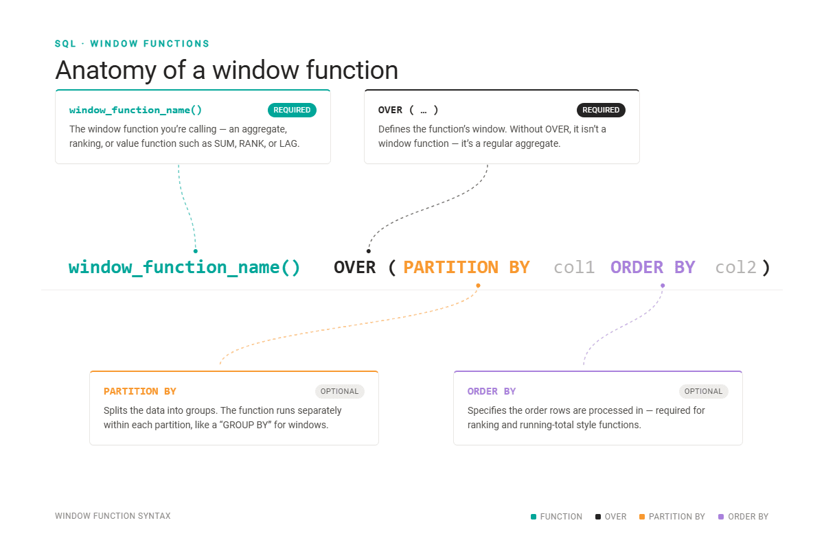
There are several important aspects of SQL window functions you need to understand when writing a window function.
Why SQL Window Functions Matter in Interviews
Here’s why: window functions are one of the most common ways interviewers separate junior candidates from senior ones.
Technically, you don’t need window functions. Most SQL problems can be solved by using subqueries, self-joins, and GROUP BY. But with window functions, you solve the same problems more elegantly and in fewer code lines. That’s what interviewers are looking for. Anyone can write working but bloated SQL code that returns the expected result.
But if you know when to use window functions and which ones to use, without the interviewer explicitly asking for them? That shows the interviewer you’ve moved beyond simply memorizing the window function syntax and started thinking in patterns. You know down to the smallest detail what a particular window function does and why it’s suitable for a certain pattern.
The 6 SQL Window Function Patterns You Need for Interviews
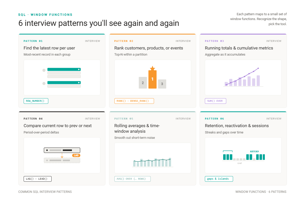
I’ll now show you how these work in practice by solving scenario-based interview questions.
Interview Pattern #1: Find the Latest Row per User
The question from Amazon and Etsy tasks you with finding the callers whose first and last calls were to the same person on a given day.
Caller History
Last Updated: October 2022
Given a phone log table that has information about callers' call history, find out the callers whose first and last calls were to the same person on a given day. Output the caller ID, recipient ID, and the date called.
Dataset
There’s a table named caller_history.
As you can see, the grain level is a call.
Solution
1. Finding the first and the last call
The most straightforward window-function approach is to use FIRST_VALUE(). As you probably suspected, that’s a window function that returns the first value – i.e., the first row – within the window.
I’ll use it to get the first call and also to get the last call, by sorting the window in descending order.
(You might ask why not use LAST_VALUE() in the latter case. Be patient, we’ll come to that. But trust me when I say that FIRST_VALUE() is your safest option.)
The data is partitioned by caller ID and call date. I apply DATE() because without it, each call would be a separate partition, since they are timestamps.
WITH first_and_last AS
  (SELECT *,
          FIRST_VALUE(recipient_id) OVER(PARTITION BY caller_id, DATE(date_called) ORDER BY date_called ASC) AS first_call,
          FIRST_VALUE(recipient_id) OVER(PARTITION BY caller_id, DATE (date_called) ORDER BY date_called DESC) AS last_call
FROM caller_history)
Be aware that window functions keep all the individual rows. So, the above SQL CTE would produce rows for every call made on a given day.
Let’s query it with a simple SELECT, so you know what I mean.
WITH first_and_last AS
  (SELECT *,
          FIRST_VALUE(recipient_id) OVER(PARTITION BY caller_id, DATE(date_called) ORDER BY date_called ASC) AS first_call,
          FIRST_VALUE(recipient_id) OVER(PARTITION BY caller_id, DATE (date_called) ORDER BY date_called DESC) AS last_call
FROM caller_history)

SELECT *
FROM first_and_last;
Here’s the output.
| caller_id | recipient_id | date_called | first_call | last_call |
|---|---|---|---|---|
| 1 | 2 | 2022-01-01 09:00:00 | 2 | 4 |
| 1 | 3 | 2022-01-01 17:00:00 | 2 | 4 |
| 1 | 4 | 2022-01-01 23:00:00 | 2 | 4 |
| 2 | 5 | 2022-07-05 09:00:00 | 5 | 3 |
| 2 | 5 | 2022-07-05 17:00:00 | 5 | 3 |
| 2 | 3 | 2022-07-05 23:00:00 | 5 | 3 |
| 2 | 5 | 2022-07-06 17:00:00 | 5 | 5 |
| 2 | 3 | 2022-08-01 09:00:00 | 3 | 3 |
| 2 | 3 | 2022-08-01 17:00:00 | 3 | 3 |
| 2 | 4 | 2022-08-02 09:00:00 | 4 | 4 |
| 2 | 5 | 2022-08-02 10:00:00 | 4 | 4 |
| 2 | 4 | 2022-08-02 11:00:00 | 4 | 4 |
2. Finding the first call by the caller
As you can see, we’re still on an analytical level. What we need to do here is find a unique combination of the columns required by the question: caller_id, recipient_id, and date_called. We again use DATE() on the date_called, because that’s also a requirement.
In the WHERE clause, we keep only the callers whose first call was to the same recipient as the last call.
Run the code above to see the output.
The Dangers of Using LAST_VALUE()
The thing is that, when you add ORDER BY to a window function, SQL quietly applies a default frame: ROWS BETWEEN UNBOUNDED PRECEDING AND CURRENT ROW. This means that the window is all the rows before the current row + the current row.
That’s fine when you use FIRST_VALUE(); the window frame includes all the preceding rows, so the first value really is the first value of the partition.
But for LAST_VALUE() – with that default window definition – the last value is actually the current row.
That’s where you can easily fail your interview, because you think just replacing FIRST_VALUE() with LAST_VALUE() to find the last call, then sorting the partition in the opposite (ascending) order, will do the trick.
No, it won’t. You can run the code above and see that the solution is incorrect.
If you really insist on using LAST_VALUE() – which I don’t recommend, as it’s easy to forget about the window frame – then you should explicitly define the window frame as UNBOUNDED FOLLOWING`. (More about window frames in the section about Interview Pattern #5.)
WITH first_and_last AS (
    SELECT *,
           FIRST_VALUE(recipient_id) OVER (PARTITION BY caller_id, DATE(date_called) ORDER BY date_called ASC) AS first_call,
           LAST_VALUE(recipient_id) OVER (PARTITION BY caller_id, DATE(date_called) ORDER BY date_called ASC ROWS BETWEEN UNBOUNDED PRECEDING AND UNBOUNDED FOLLOWING) AS last_call
    FROM caller_history
)

SELECT DISTINCT caller_id,
                first_call AS recipient,
                DATE(date_called)
FROM first_and_last
WHERE first_call = last_call;
Safer Alternative: ROW_NUMBER()
Another way of solving this problem is to use ROW_NUMBER() instead of FIRST_VALUE().
While FIRST_VALUE() is a more elegant solution, you should also know how to use ROW_NUMBER() in this pattern. And when. Which is when you need the full row, need to handle ties deliberately, or need to operate on the first and last groups as separate datasets.
Here’s the interview question solution rewritten with ROW_NUMBER().
This window function assigns unique integers to each row within a partition. You rank them from the first to the last call, then from the last to the first call.
Then, in separate CTEs, keep only rows where the row number is 1; those are your first and last calls.
Finally, join those two CTEs on the caller_id, call_date, and recipient_id, and there you have it.
WITH ranked AS (
    SELECT *,
           ROW_NUMBER() OVER (PARTITION BY caller_id, DATE(date_called)
                              ORDER BY date_called ASC)  AS rn_first,
           ROW_NUMBER() OVER (PARTITION BY caller_id, DATE(date_called)
                              ORDER BY date_called DESC) AS rn_last
    FROM caller_history
),
first_calls AS (
    SELECT caller_id, recipient_id, DATE(date_called) AS call_date
    FROM ranked
    WHERE rn_first = 1
),
last_calls AS (
    SELECT caller_id, recipient_id, DATE(date_called) AS call_date
    FROM ranked
    WHERE rn_last = 1
)
SELECT f.caller_id,
       f.recipient_id,
       f.call_date
FROM first_calls f
JOIN last_calls l
    ON  f.caller_id  = l.caller_id
    AND f.call_date  = l.call_date
    AND f.recipient_id = l.recipient_id;
Interview Pattern #2: Rank Customers, Products, or Events
Ranking is another popular interview pattern and typically calls for using one of these functions.
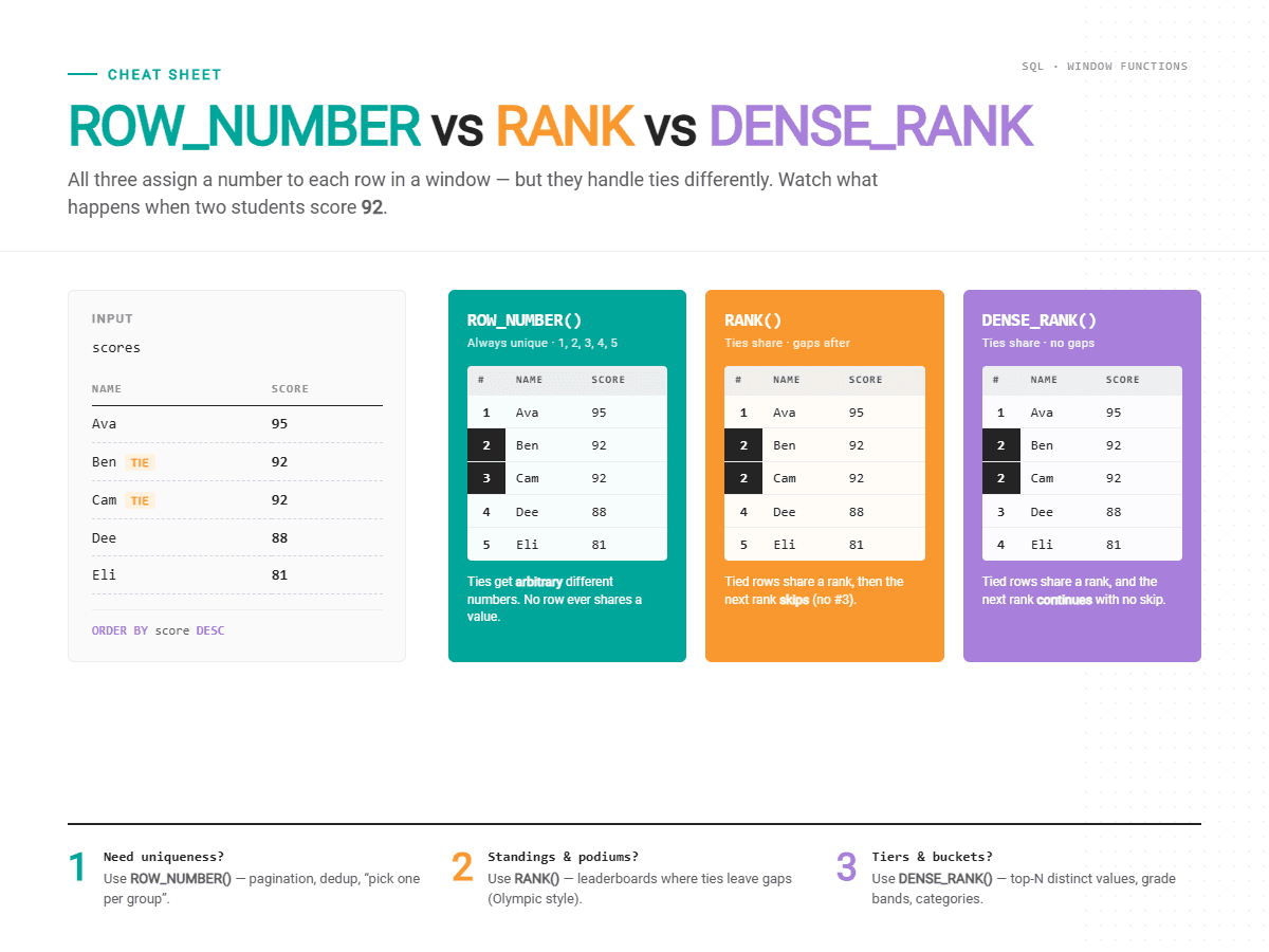
As for the practical use, let’s solve this interview question from the City of San Francisco.
We need to find the top two highest-paid City employees for each job title, ranked by total pay and benefits. The output should include the job title and the names of the highest- and second-highest-paid employees.
Highest Paid City Employees
Find the top 2 highest paid city employees for each job title. Rank employees by their total compensation. Output each job title along with the corresponding highest and second-highest paid employees.
If multiple employees are tied within the same job title, return the employee whose name comes last alphabetically.
Dataset
We’re working with the table named sf_public_salaries.
Solution
1. Ranking employees on their total pay and benefits
We must use ROW_NUMBER() in the solution. Why? We now know that it assigns unique integers, even if there are rows with the same value, i.e., duplicates.
OK, but the question never explicitly says which ranking window function to use. Of course it doesn’t; it’s an interview question! Do you think your boss will hold your hand and tell you which function to use? No, ‘course not! You have to decide on your own.
The key to this interview question is in the expectation that exactly one employee lands in position 1 and exactly one in position 2. Different positions, even if they have the same salary + benefits? That sounds like a job for ROW_NUMBER().
We use it to query employees, their job titles and total benefits, and to rank them from highest to lowest total benefits. The ranking is for each job title separately; that’s why I partitioned the data.
SELECT employeename,
       jobtitle,
       totalpaybenefits,
       ROW_NUMBER() OVER (PARTITION BY jobtitle ORDER BY totalpaybenefits DESC) AS pos
FROM sf_public_salaries
As a standalone query, it gives you this output. You can see that employees within each job title are ranked separately.
| employeename | jobtitle | totalpaybenefits | pos |
|---|---|---|---|
| PATRICIA JACKSON | CAPTAIN III (POLICE DEPARTMENT) | 297608.92 | 1 |
| ANNA BROWN | CAPTAIN III (POLICE DEPARTMENT) | 238551.88 | 2 |
| DOUGLAS MCEACHERN | CAPTAIN III (POLICE DEPARTMENT) | 196494.14 | 3 |
| JOHN LOFTUS | CAPTAIN III (POLICE DEPARTMENT) | 192951.37 | 4 |
| TERESA BARRETT | CAPTAIN III (POLICE DEPARTMENT) | 192914.5 | 5 |
| Lance A Obtinalla Jr | Deputy Sheriff | 137519.28 | 1 |
| Arnel Maracha | Deputy Sheriff | 137235.94 | 2 |
| Patrick T Truong | Deputy Sheriff | 136478.65 | 3 |
| Yvette R Gay | Deputy Sheriff | 135221.29 | 4 |
| Petra Hahn | Deputy Sheriff | 135073.93 | 5 |
| Donald V Ortiz | Deputy Sheriff | 134987.81 | 6 |
| Theresa Courtney | Deputy Sheriff | 133147.67 | 7 |
| Stephen Kendall | Deputy Sheriff | 131854.1 | 8 |
| Patrick Crane | Deputy Sheriff | 129599.94 | 9 |
| Rizaldy T Tabada | Deputy Sheriff | 129071.16 | 10 |
| Ceasar Garcia | Deputy Sheriff | 127283.35 | 11 |
| Otha Cotton | Deputy Sheriff | 126856.84 | 12 |
| Patrick T Truong | Deputy Sheriff | 125480.95 | 13 |
| Aaron Schmidt | Deputy Sheriff | 124012.63 | 14 |
| Sarah Silva | Deputy Sheriff | 123079.67 | 15 |
| Richard Kendall | Deputy Sheriff | 122344.8 | 16 |
| Robert J Loberg | Deputy Sheriff | 119079.59 | 17 |
| Brian E Oconnor | Deputy Sheriff | 11175.91 | 18 |
| Kenia C Coronado | Eligibility Worker | 55429.49 | 1 |
| Tretha T Stroughter | Eligibility Worker | 38346.82 | 2 |
| Mary R Carr | Eligibility Worker | 37903.05 | 3 |
| Barry Hyun | Eligibility Worker | 35101.86 | 4 |
| Arturo Galarza | Eligibility Worker | 32276.85 | 5 |
| Daniel Phillip Boutote | Eligibility Worker | 24378.44 | 6 |
| Heather E Gutierres | Eligibility Worker | 6339.27 | 7 |
| Mandisa Mabrey | Eligibility Worker | 3572.42 | 8 |
| Melinda Kuoch | Eligibility Worker | 2439.06 | 9 |
| Claire M Leflore | Eligibility Worker | 2013.94 | 10 |
| Shickola Ricks | Eligibility Worker | 1634.69 | 11 |
| Alexander M Lamond | EMT/Paramedic/Firefighter | 139818.1 | 1 |
| Teresa L Cavanaugh | EMT/Paramedic/Firefighter | 139524.66 | 2 |
| Jared F Cooper | EMT/Paramedic/Firefighter | 132354.45 | 3 |
| Michael Mason | EMT/Paramedic/Firefighter | 131679.7 | 4 |
| Graham P Hoffman | EMT/Paramedic/Firefighter | 128504.14 | 5 |
| Thomas Ro | EMT/Paramedic/Firefighter | 125213.2 | 6 |
| Ryan J Jamison | EMT/Paramedic/Firefighter | 117370.71 | 7 |
| Jason L Landivar | EMT/Paramedic/Firefighter | 116936.65 | 8 |
| Patrick S Renshaw | EMT/Paramedic/Firefighter | 114467.01 | 9 |
| James Lockhart | EMT/Paramedic/Firefighter | 79674.55 | 10 |
| Nicole J Lafata Shark | EMT/Paramedic/Firefighter | 56376.86 | 11 |
| Christina A Couch | EMT/Paramedic/Firefighter | 48397.69 | 12 |
| Neal K Rodil | EMT/Paramedic/Firefighter | 47402.38 | 13 |
| Emily Anderson | EMT/Paramedic/Firefighter | 45310.01 | 14 |
| Sherry Mahoney | EMT/Paramedic/Firefighter | 43766.89 | 15 |
| Seaborn Chiles | EMT/Paramedic/Firefighter | 43628.56 | 16 |
| Andrew G Chen | Estate Investigator | 113849.01 | 1 |
| Grace Lin | Estate Investigator | 113066.8 | 2 |
| Patrick Martinez | Estate Investigator | 110648.97 | 3 |
| Denise Alexander | Estate Investigator | 92145.7 | 4 |
| Gregory B Bovo | Firefighter | 33739.71 | 1 |
| Ryan C Crow | Firefighter | 33739.71 | 2 |
| Ernest E Hayles | Firefighter | 15752.32 | 3 |
| Elizabeth M Leahy | Firefighter | 1886.38 | 4 |
| Kari A Johnson | Firefighter | 832.1 | 5 |
| NATHANIEL FORD | GENERAL MANAGER-METROPOLITAN TRANSIT AUTHORITY | 567595.43 | 1 |
| EDWARD REISKIN | GENERAL MANAGER-METROPOLITAN TRANSIT AUTHORITY | 230827.12 | 2 |
| Dennis J Gerbino | IS Programmer Analyst | 96972.32 | 1 |
| Clark Bell | IS Programmer Analyst-Senior | 95399.5 | 1 |
| Melinda Wong | Junior Administrative Analyst | 81039.65 | 1 |
| Natalia Y Castillo Villegas | Junior Administrative Analyst | 80020.19 | 2 |
| Francis J Monsada | Junior Administrative Analyst | 79948.2 | 3 |
| LEA YAMAGATA | LIBRARY PAGE | 17064.42 | 1 |
| Nina Davis | PS Aide Health Services | 9694.34 | 1 |
| Ray Torres | Public Service Trainee | 1307.05 | 1 |
| Alondra Correa Almanza | Public Service Trainee | 1117.7 | 2 |
| Jack O'Sullivan | Public Service Trainee | 1079.42 | 3 |
| Eric J Chen | Public Service Trainee | 844.14 | 4 |
| Patrick F Mcpartland | Public Service Trainee | 506.14 | 5 |
| Darrel A Lachapelle | Public Service Trainee | 323.2 | 6 |
| Sophia Wu | Public Service Trainee | 298.36 | 7 |
| Jimmy Tang | Public Service Trainee | 184.41 | 8 |
| Pecola Jones | Public Svc Aide-Public Works | 4972.34 | 1 |
| Roy Hill | Public Svc Aide-Public Works | 2684.01 | 2 |
| Alicia Brown | Public Svc Aide-Public Works | 2597.32 | 3 |
| Kevin Clark | Public Svc Aide-Public Works | 2542.05 | 4 |
| Antionette L Riley | Public Svc Aide-Public Works | 2420.18 | 5 |
| Clarence Walker | Public Svc Aide-Public Works | 2375.72 | 6 |
| Maiza Padilla | Public Svc Aide-Public Works | 2371.01 | 7 |
| Willie Collins | Public Svc Aide-Public Works | 2363.91 | 8 |
| Mario Armbrister | Public Svc Aide-Public Works | 2250.06 | 9 |
| Jesus J Aromin | Public Svc Aide-Public Works | 2144.7 | 10 |
| Alan K Tolbert | Public Svc Aide-Public Works | 2090.99 | 11 |
| Orlando M Gonzalez | Public Svc Aide-Public Works | 2006.96 | 12 |
| Fernando Barajas | Public Svc Aide-Public Works | 1763.67 | 13 |
| Arnitial Donely | Public Svc Aide-Public Works | 1623.19 | 14 |
| Ivan Y Castillo | Public Svc Aide-Public Works | 1613.88 | 15 |
| David Ayers Jr | Public Svc Aide-Public Works | 1560.11 | 16 |
| Iesha M Jones | Public Svc Aide-Public Works | 1558.4 | 17 |
| Glenn Daniels | Public Svc Aide-Public Works | 1138.8 | 18 |
| Jose F Granados | Public Svc Aide-Public Works | 667.81 | 19 |
| Marcus Duty | Public Svc Aide-Public Works | 578.19 | 20 |
| Silas D Moultrie Jr | Public Svc Aide-Public Works | 322.21 | 21 |
| Andre Thomas | Public Svc Aide-Public Works | 172.13 | 22 |
| Brighton M Leung | Public Svc Aide-Public Works | 108.43 | 23 |
| Sara Paredes | Registered Nurse | 89513.97 | 1 |
| Emilia C Patrick | Registered Nurse | 87357.27 | 2 |
| Kathryn L Fowler | Registered Nurse | 86194.27 | 3 |
| Raffaella V Wilson | Registered Nurse | 78763.72 | 4 |
| Adina M Diamond | Registered Nurse | 77879.37 | 5 |
| Mary C Huston | Registered Nurse | 77834.88 | 6 |
| Karen M Gomez | Registered Nurse | 68013.87 | 7 |
| Ying Ying Hui | Registered Nurse | 60078.4 | 8 |
| Christopher Wilcox | Registered Nurse | 49366.55 | 9 |
| Lilly Fung | Registered Nurse | 38692.45 | 10 |
| Beverly Bagdorf | Registered Nurse | 32809.65 | 11 |
| Mo Ching Wan | Registered Nurse | 29364.77 | 12 |
| Jeanne M D'Arcy | Registered Nurse | 29212.95 | 13 |
| Audrey Ngo | Registered Nurse | 23237.16 | 14 |
| Margarita Herrera | Registered Nurse | 22320.13 | 15 |
| Liane Angus | Registered Nurse | 11499.04 | 16 |
| Robert Martinez | Registered Nurse | 9969.11 | 17 |
| Joann G Siobal | Registered Nurse | 7959.18 | 18 |
| Leanne Abrigo Johnson | Registered Nurse | 4891.07 | 19 |
| Linda Pizzorno | Registered Nurse | 1025.65 | 20 |
| Renato C Gurion | Registered Nurse | 7.24 | 21 |
| Frankie Johnson | Senior Eligibility Worker | 100795.02 | 1 |
| YEVA JOHNSON | SENIOR PHYSICIAN SPECIALIST | 178760.58 | 1 |
| Mark F Obrochta | Sergeant 3 | 195887.06 | 1 |
| Kathryn Waaland | Sergeant 3 | 189864.25 | 2 |
| Lawrence Chan | Sergeant 3 | 189689.57 | 3 |
| Joseph M Salazar | Sergeant 3 | 186630.42 | 4 |
| Melonee Alvarez | Sergeant 3 | 186535.52 | 5 |
| Steven Stocker | Sergeant 3 | 186479.79 | 6 |
| Omar Bueno | Sergeant 3 | 185627.05 | 7 |
| Patrick Kennedy | Sergeant 3 | 177603.94 | 8 |
| Ernanie Rasquero | Special Nurse | 2739.94 | 1 |
| Paul J Ortiz | Special Nurse | 2463.16 | 2 |
| Elizabeth J Dayrit | Special Nurse | 2334.2 | 3 |
| Emilia C Patrick | Special Nurse | 2198.09 | 4 |
| Yolanda Ramirez | Special Nurse | 2129.09 | 5 |
| Ayala Mirande | Special Nurse | 1743.18 | 6 |
| David Fleming | Special Nurse | 1729.84 | 7 |
| Jamie J Dwyer | Special Nurse | 1673.38 | 8 |
| Jessica H Lee | Special Nurse | 1517.16 | 9 |
| Russell Patrick Mangahas | Special Nurse | 1431.53 | 10 |
| Justina Dizon | Special Nurse | 1368.06 | 11 |
| Juliet Palarca | Special Nurse | 1265.32 | 12 |
| John Donnelly | Special Nurse | 1232.32 | 13 |
| Alma Rosa Garcia | Special Nurse | 1069.04 | 14 |
| David A Fleming | Special Nurse | 777.18 | 15 |
| Reuben Reyes | Special Nurse | 726.53 | 16 |
| Carla R Greenblatt | Special Nurse | 652.2 | 17 |
| Catheryn Williams | Special Nurse | 474.54 | 18 |
| Graciela M Arevalo | Special Nurse | 350.39 | 19 |
| Connie Love-Miles | Special Nurse | 332.23 | 20 |
| Blesilda P Huypungco | Special Nurse | 137.94 | 21 |
| Vanessa E Almaguer | Special Nurse | 88.18 | 22 |
| Grace Salud | Special Nurse | 46.27 | 23 |
| Merter Bozkurt | Transit Operator | 43295.64 | 1 |
| Matthew Lu | Transit Operator | 40864.94 | 2 |
| Terry L Johnson | Transit Operator | 38919.75 | 3 |
| Sedrick M Mcarthur | Transit Operator | 36883.76 | 4 |
| Alvin Sosa | Transit Operator | 31625.88 | 5 |
| Pelzie L Smith | Transit Operator | 28403.95 | 6 |
| Linda Edwards | Transit Operator | 28298.63 | 7 |
| Dhakir R Zaki | Transit Operator | 27572.32 | 8 |
| Miguel J Gonzalez Jr | Transit Operator | 25922.1 | 9 |
| Wallina C Pellette | Transit Operator | 24211.81 | 10 |
| Nicole Freeney | Transit Operator | 22228.39 | 11 |
| Annette Kess | Transit Operator | 19767.18 | 12 |
| Emmanuel R Borja | Transit Operator | 19110 | 13 |
| Victor N Yeung | Transit Operator | 18175.28 | 14 |
| Tim C Ghigliazza | Transit Operator | 17821.35 | 15 |
| Tara A Amado | Transit Operator | 17271.75 | 16 |
| Niem Tran | Transit Operator | 14982.84 | 17 |
| George L Abrams Jr | Transit Operator | 13713 | 18 |
| Marie E Monsen | Transit Operator | 13544.03 | 19 |
| Luana D Beavers-Deloach | Transit Operator | 13142.65 | 20 |
| Larry J Davis | Transit Operator | 13036.05 | 21 |
| Terri L Mathis | Transit Operator | 12023.9 | 22 |
| Michaela T Womack | Transit Operator | 11943.29 | 23 |
| Willie Daigle Jr | Transit Operator | 11916.08 | 24 |
| Monique C Jacobs | Transit Operator | 11808.51 | 25 |
| Samer Bouri | Transit Operator | 8794.53 | 26 |
| Ben D Malone | Transit Operator | 8681.42 | 27 |
| Carolyn E Robinson | Transit Operator | 8675.21 | 28 |
| Lawrence C Blakes Jr | Transit Operator | 8562.44 | 29 |
| Jarrett L Louie | Transit Operator | 8554.71 | 30 |
| Robert E Lee Jr | Transit Operator | 8505.11 | 31 |
| John Hunt | Transit Operator | 8493.27 | 32 |
| George Fudge | Transit Operator | 8308.31 | 33 |
| Ira Newman | Transit Operator | 8074.9 | 34 |
| Tracy Y Higgins | Transit Operator | 8014.34 | 35 |
| Georgina M Pineda | Transit Operator | 7959.18 | 36 |
| Gwen Ferdinand | Transit Operator | 7751.47 | 37 |
| Jacquelyn Vassar | Transit Operator | 6953.83 | 38 |
| Wing C Kwan | Transit Operator | 5617.43 | 39 |
| Lenora Hamilton | Transit Operator | 3993.87 | 40 |
| Kennis Grant | Transit Operator | 3618.66 | 41 |
| Vivian A Showers | Transit Operator | 3038.44 | 42 |
| Darryl L Armstrong | Transit Operator | 2500.86 | 43 |
| Sen Cheong Lai | Transit Operator | 1164.91 | 44 |
| Iris J Lett | Transit Operator | 1150.71 | 45 |
| Joannie Keys | Transit Operator | 1127.22 | 46 |
| Maria E Zuniga | Transit Operator | 114.54 | 47 |
Scroll down a little until you reach firefighters. You’ll see ROW_NUMBER() doing its magic: Gregory B Bovo and Ryan C Crow – those must be real names! – have the same total compensation, but they have different ranks. How does it decide which gets which rank? It’s up to the database engine to decide, meaning ROW_NUMBER() is non-deterministic. Yes, run the query the second time, and you might get different results. For this task, it doesn’t really matter. It seems our engine decided to rank alphabetically when total benefits were the same; that’s perfectly fine.
2. Selecting only employees ranked as 1 and 2
In the next step, we turn the above query into a subquery. The outer query uses it to select only the first- and second-ranked employees, then uses CASE WHEN to assign a separate column to each employee. I named those columns primus and secundum. Why not flex your Latin?
SELECT jobtitle,
       CASE
           WHEN pos = 1 THEN employeename
           ELSE NULL
       END AS primus,
       CASE
           WHEN pos = 2 THEN employeename
           ELSE NULL
       END AS secundum
FROM
   (SELECT employeename,
           jobtitle,
           totalpaybenefits,
           ROW_NUMBER() OVER (PARTITION BY jobtitle ORDER BY totalpaybenefits DESC) AS pos
      FROM sf_public_salaries) one
WHERE pos <= 2
Here’s what the output looks like, so you get the feeling of what we’re doing here. That output is basically it; all the info we need is there. Only, we have to make it more readable, as there’s no need to have duplicate job title rows.
| jobtitle | primus | secundum |
|---|---|---|
| CAPTAIN III (POLICE DEPARTMENT) | PATRICIA JACKSON | |
| CAPTAIN III (POLICE DEPARTMENT) | ANNA BROWN | |
| Deputy Sheriff | Lance A Obtinalla Jr | |
| Deputy Sheriff | Arnel Maracha | |
| Eligibility Worker | Kenia C Coronado | |
| Eligibility Worker | Tretha T Stroughter | |
| EMT/Paramedic/Firefighter | Alexander M Lamond | |
| EMT/Paramedic/Firefighter | Teresa L Cavanaugh | |
| Estate Investigator | Andrew G Chen | |
| Estate Investigator | Grace Lin | |
| Firefighter | Gregory B Bovo | |
| Firefighter | Ryan C Crow | |
| GENERAL MANAGER-METROPOLITAN TRANSIT AUTHORITY | NATHANIEL FORD | |
| GENERAL MANAGER-METROPOLITAN TRANSIT AUTHORITY | EDWARD REISKIN | |
| IS Programmer Analyst | Dennis J Gerbino | |
| IS Programmer Analyst-Senior | Clark Bell | |
| Junior Administrative Analyst | Melinda Wong | |
| Junior Administrative Analyst | Natalia Y Castillo Villegas | |
| LIBRARY PAGE | LEA YAMAGATA | |
| PS Aide Health Services | Nina Davis | |
| Public Service Trainee | Ray Torres | |
| Public Service Trainee | Alondra Correa Almanza | |
| Public Svc Aide-Public Works | Pecola Jones | |
| Public Svc Aide-Public Works | Roy Hill | |
| Registered Nurse | Sara Paredes | |
| Registered Nurse | Emilia C Patrick | |
| Senior Eligibility Worker | Frankie Johnson | |
| SENIOR PHYSICIAN SPECIALIST | YEVA JOHNSON | |
| Sergeant 3 | Mark F Obrochta | |
| Sergeant 3 | Kathryn Waaland | |
| Special Nurse | Ernanie Rasquero | |
| Special Nurse | Paul J Ortiz | |
| Transit Operator | Merter Bozkurt | |
| Transit Operator | Matthew Lu |
3. Grouping the data and finding the first- and second-ranked employees
Now, the final step: all the previous code becomes another subquery, embedded in an outer query. I use MAX() and GROUP BY to collapse two rows into a single row. Don’t worry, MAX() doesn’t perform any meaningful “maximum” calculation here. It’s just a trick I use to extract the single non-NULL value per group; MIN() would work, too.
Here’s the whole code.
Run the code above to see the output.
Why Do RANK() & DENSE_RANK() Fail Here?
Let’s go back to our first subquery, the one where all the ranking occurs. I’ve changed it slightly by adding RANK() and DENSE_RANK() and keeping only the firefighter job title (only for educational purposes); that’s where there are employees with the same total salary.
SELECT employeename,
       jobtitle,
       totalpaybenefits,
       ROW_NUMBER() OVER (PARTITION BY jobtitle ORDER BY totalpaybenefits DESC) AS row_number_pos,
       RANK() OVER (PARTITION BY jobtitle ORDER BY totalpaybenefits DESC) AS rank_pos,
       DENSE_RANK() OVER (PARTITION BY jobtitle ORDER BY totalpaybenefits DESC) AS dense_rank_pos
FROM sf_public_salaries
WHERE jobtitle = 'Firefighter'
Here is what you get.
| employeename | jobtitle | totalpaybenefits | row_number_pos | rank_pos | dense_rank_pos |
|---|---|---|---|---|---|
| Gregory B Bovo | Firefighter | 33739.71 | 1 | 1 | 1 |
| Ryan C Crow | Firefighter | 33739.71 | 2 | 1 | 1 |
| Ernest E Hayles | Firefighter | 15752.32 | 3 | 3 | 2 |
| Elizabeth M Leahy | Firefighter | 1886.38 | 4 | 4 | 3 |
| Kari A Johnson | Firefighter | 832.1 | 5 | 5 | 4 |
With RANK(), those two employees with the same total salary will both be ranked as 1. Even if we pick the correct first-ranked employee, this method doesn’t assign a rank 2, so the second_best column in the final code will be empty. That’s, of course, incorrect.
As for DENSE_RANK(), the first part of the problem is the same; both employees are ranked as 1. However, there is an employee ranked as 2, which is great. But, it’s Ernest E Hayles, which is, again, incorrect.
You see where I’m going with this? Let’s see the final code with either method, and let’s keep only firefighters.
Here’s RANK().
SELECT jobtitle,
       MAX(primus) AS best,
       MAX(secundum) AS second_best
FROM
  (SELECT jobtitle,
          CASE
              WHEN pos = 1 THEN employeename
              ELSE NULL
          END AS primus,
          CASE
              WHEN pos = 2 THEN employeename
              ELSE NULL
          END AS secundum
   FROM
     (SELECT employeename,
             jobtitle,
             totalpaybenefits,
             RANK() OVER (PARTITION BY jobtitle
                                ORDER BY totalpaybenefits DESC) AS pos

      FROM sf_public_salaries
      WHERE jobtitle = 'Firefighter') one
   WHERE pos <= 2) two
GROUP BY jobtitle;
As I predicted, the second_best column is empty. This is why using RANK() here would make you fail the interview.
| jobtitle | best | second_best |
|---|---|---|
| Firefighter | Ryan C Crow |
Here’s the same thing, but with DENSE_RANK().
SELECT jobtitle,
       MAX(primus) AS best,
       MAX(secundum) AS second_best
FROM
  (SELECT jobtitle,
          CASE
              WHEN pos = 1 THEN employeename
              ELSE NULL
          END AS primus,
          CASE
              WHEN pos = 2 THEN employeename
              ELSE NULL
          END AS secundum
   FROM
     (SELECT employeename,
             jobtitle,
             totalpaybenefits,
             DENSE_RANK() OVER (PARTITION BY jobtitle
                                ORDER BY totalpaybenefits DESC) AS pos

      FROM sf_public_salaries
      WHERE jobtitle = 'Firefighter') one
   WHERE pos <= 2) two
GROUP BY jobtitle;
You can see in the output that the best and the second-best employees are incorrect. Gregory B Bovo and Ryan C Crow should be there. Instead, we got Ernest E Hayles. That’s the reason why you can’t use DENSE_RANK(), either.
| jobtitle | best | second_best |
|---|---|---|
| Firefighter | Ryan C Crow | Ernest E Hayles |
Interview Pattern #3: Calculate Running Totals and Cumulative Metrics
Running totals and cumulative metrics in general are calculated using the SUM() window function with the ORDER BY clause in OVER().
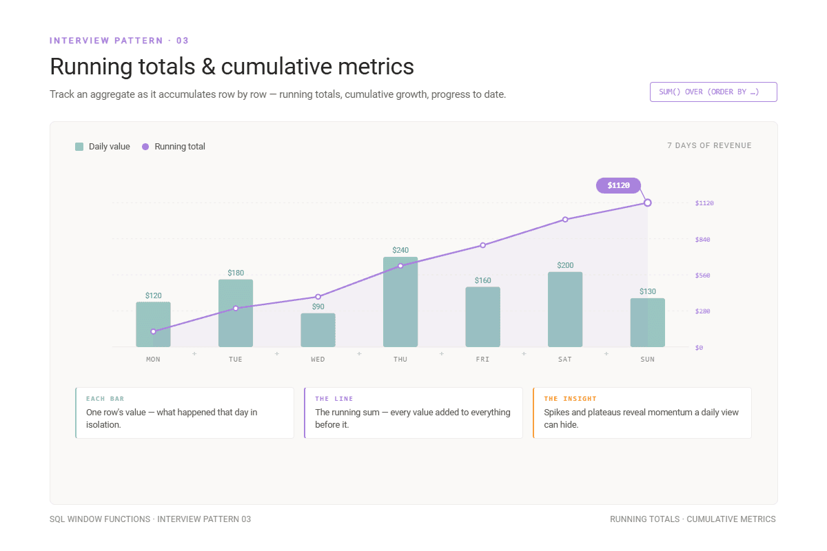
I’ll demonstrate this with the interview question from Goldman Sachs and Deloitte.
Minimum Number of Platforms
Last Updated: December 2021
You are given a day worth of scheduled departure and arrival times of trains at one train station. One platform can only accommodate one train from the beginning of the minute it's scheduled to arrive until the end of the minute it's scheduled to depart. Find the minimum number of platforms necessary to accommodate the entire scheduled traffic.
You’re given one day’s data about trains’ departures and arrivals at one train station. You need to find the minimum number of platforms necessary to accommodate the entire scheduled traffic. All that knowing that one platform can only accommodate one train at a time, i.e., from its arrival until its departure time.
Dataset
There are two tables; the first one is train_arrivals.
The second table is, as expected, train_departures.
Solution
In the CTE, we chain two SELECT statements: the first one marks the train’s arrival as 1, the second one marks its departure as -1. With UNION ALL, we merge the results of both statements into a single dataset.
1. Combine arrivals and departures in one dataset
The result is sorted by time in ascending order and by mark in descending order; in case of ties, arrivals are considered before departures.
WITH timetable AS(
    (SELECT train_id,
            arrival_time AS time,
            1 AS mark
     FROM train_arrivals

     UNION ALL

     SELECT train_id,
            departure_time AS time,
            -1 AS mark
     FROM train_departures
     )
    ORDER BY time ASC, mark DESC),
Here’s what the data looks like now.
| train_id | time | mark |
|---|---|---|
| 1 | 08:00 | 1 |
| 2 | 08:05 | 1 |
| 3 | 08:05 | 1 |
| 4 | 08:10 | 1 |
| 5 | 08:10 | 1 |
| 2 | 08:10 | -1 |
| 1 | 08:15 | -1 |
| 5 | 08:20 | -1 |
| 3 | 08:20 | -1 |
| 4 | 08:25 | -1 |
| 6 | 12:15 | 1 |
| 7 | 12:20 | 1 |
| 8 | 12:25 | 1 |
| 7 | 12:25 | -1 |
| 8 | 12:30 | -1 |
| 6 | 13:00 | -1 |
| 10 | 15:00 | 1 |
| 11 | 15:00 | 1 |
| 9 | 15:00 | 1 |
| 9 | 15:05 | -1 |
| 12 | 15:06 | 1 |
| 10 | 15:10 | -1 |
| 11 | 15:15 | -1 |
| 12 | 15:15 | -1 |
| 13 | 20:00 | 1 |
| 14 | 20:10 | 1 |
| 13 | 20:15 | -1 |
| 14 | 20:15 | -1 |
2. Calculating the cumulative sum
Next, we add another CTE where we calculate the running totals. In this case, it’s not cumulative revenue, but a cumulative number of trains waiting at the station at the same time. This will give us the answer to the interview question.
The cumulative is calculated using the SUM() window function and summing marks (i.e., departures and arrivals) from the earliest to the latest time. This is the core principle of cumulative metrics. You can’t sum just any random time periods one after the other; the time data has to be sorted in ascending order.
In addition, we sort the window by mark in descending order. This is to handle the tie-breaking edge case, when a train arrives, and another train departs at the exact same time.
Let’s clarify this. Here’s what happens in the edge case if we first process the departure.
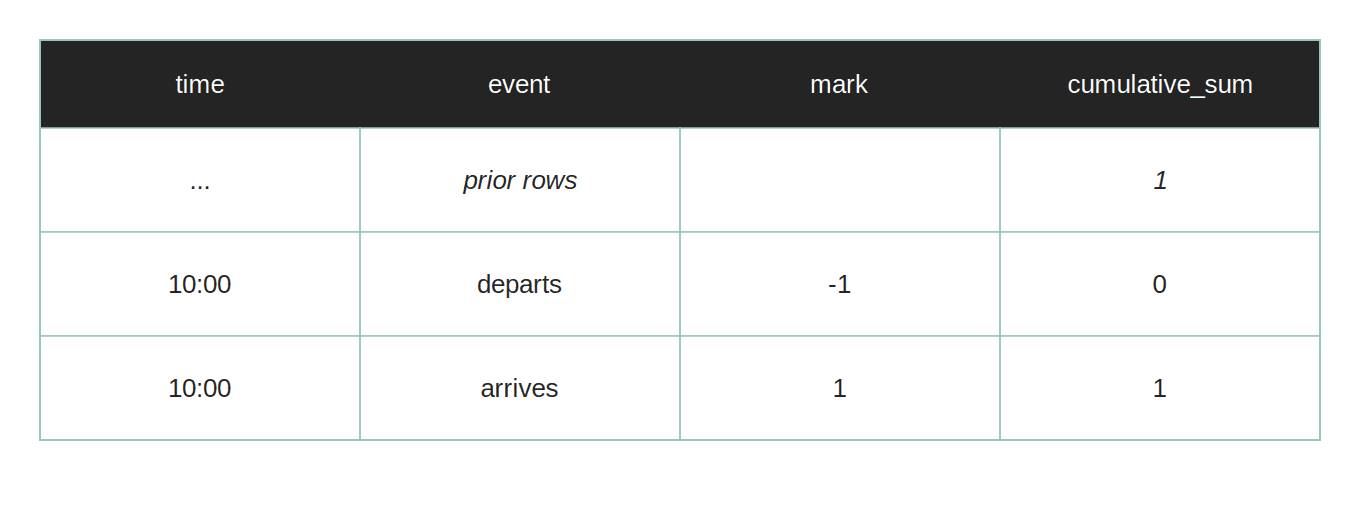
This says that we need only one platform to accommodate these two trains. But that doesn’t make sense, because the first train hadn’t yet left when the second train should have already arrived. We know that one platform can accommodate only one train.
Therefore, we have to process arrivals first, which will increase the cumulative number of trains like this.
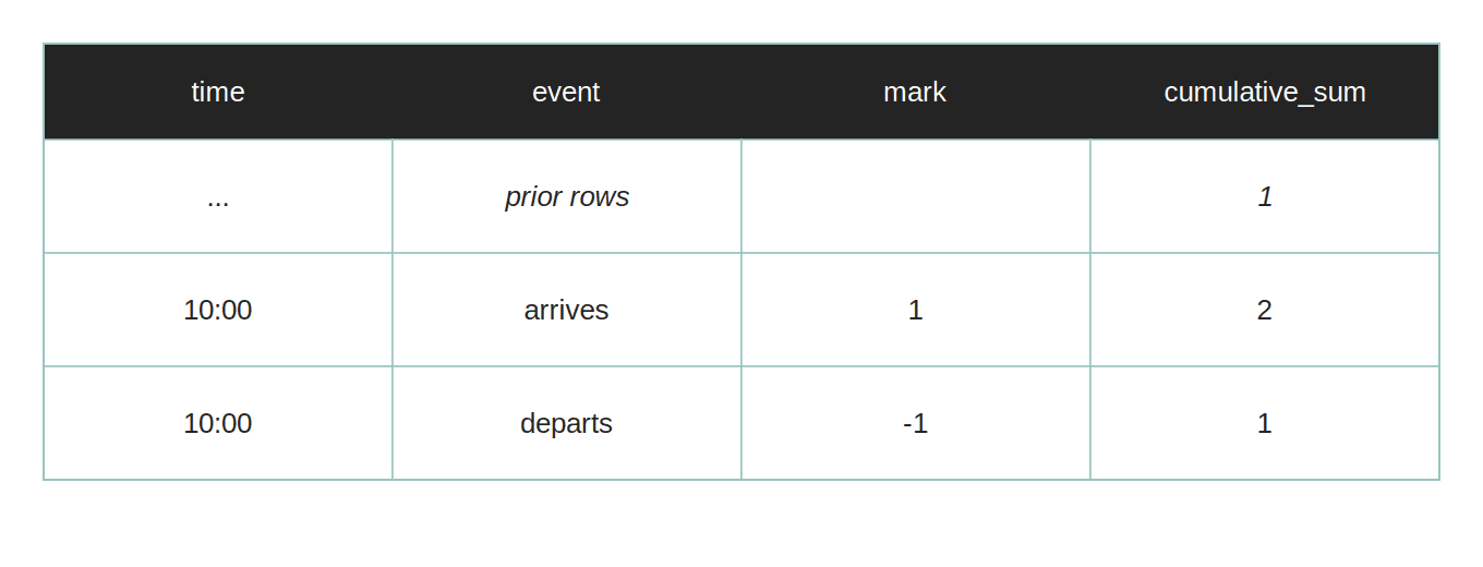
The cumulative sum peaks at two. That’s correct, we need two platforms for those two trains.
So, back to our query. By adding the cumsum CTE…
cumsum AS
  (SELECT *,
          SUM(mark) OVER (ORDER BY time ASC, mark DESC) AS trains_at_same_time
   FROM timetable
   )
…we get this output. It’s an overview of the number of platforms for each train’s departure and arrival.
| train_id | time | mark | trains_at_same_time |
|---|---|---|---|
| 1 | 08:00 | 1 | 1 |
| 2 | 08:05 | 1 | 3 |
| 3 | 08:05 | 1 | 3 |
| 4 | 08:10 | 1 | 5 |
| 5 | 08:10 | 1 | 5 |
| 2 | 08:10 | -1 | 4 |
| 1 | 08:15 | -1 | 3 |
| 5 | 08:20 | -1 | 1 |
| 3 | 08:20 | -1 | 1 |
| 4 | 08:25 | -1 | 0 |
| 6 | 12:15 | 1 | 1 |
| 7 | 12:20 | 1 | 2 |
| 8 | 12:25 | 1 | 3 |
| 7 | 12:25 | -1 | 2 |
| 8 | 12:30 | -1 | 1 |
| 6 | 13:00 | -1 | 0 |
| 10 | 15:00 | 1 | 3 |
| 11 | 15:00 | 1 | 3 |
| 9 | 15:00 | 1 | 3 |
| 9 | 15:05 | -1 | 2 |
| 12 | 15:06 | 1 | 3 |
| 10 | 15:10 | -1 | 2 |
| 11 | 15:15 | -1 | 0 |
| 12 | 15:15 | -1 | 0 |
| 13 | 20:00 | 1 | 1 |
| 14 | 20:10 | 1 | 2 |
| 13 | 20:15 | -1 | 0 |
| 14 | 20:15 | -1 | 0 |
3. Aggregation and the final output
The only thing remaining is to aggregate that into a single number using MAX() to find the maximum cumulative value, which is – I know this might sound contradictory – the minimum number of platforms necessary to accommodate the entire scheduled traffic.
So, here’s the complete solution.
Here’s the output.
| min_platforms |
|---|
| 5 |
Interview Pattern #4: Compare the Current Row to the Previous or Next Row
For this pattern, the two main window functions you’ll need are LAG() and LEAD().
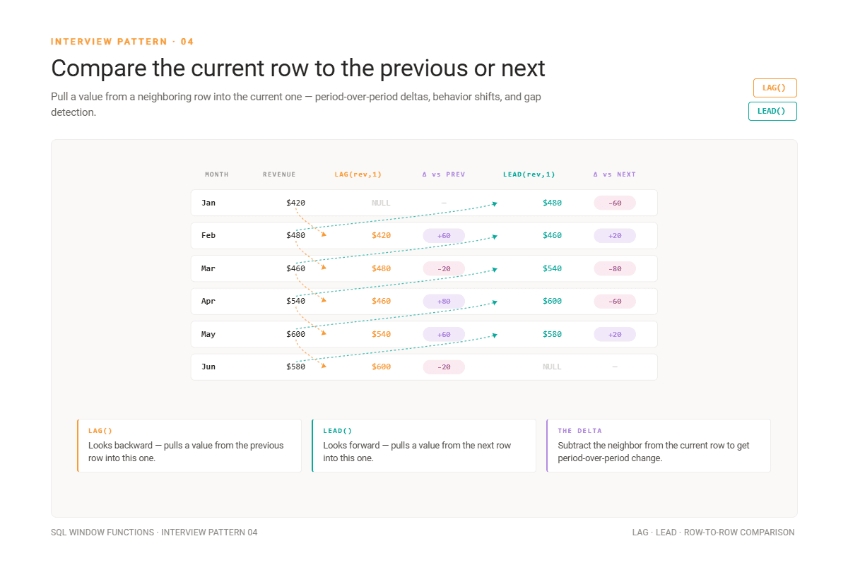
This question by ESPN is a great example of this pattern in practice.
Find how the average male height changed between each Olympics from 1896 to 2016
Find how the average male height changed between each Olympics from 1896 to 2016. Output the Olympics year, average height, previous average height, and the corresponding average height difference. Order records by the year in ascending order.
If avg height for some year is not found, assume that the average height of athletes for that year is 172.73.
You need to find how the average male height changed between the Olympics from 1896 to 2016. The output should consist of the Olympics year, the average height, the previous Olympics’ average height, and the height difference between the two years.
The question also states that the average height is 172.73 if there’s no average height for that year.
Dataset
You’re given the olympics_athletes_events table.
Solution
How would you solve this problem? By reading the question’s requirements, you should notice that we’re comparing the current year with the previous year. That should signal to you that LAG() is appropriate.
Let’s approach this systematically.
The only non-calculated column that’s required in the output is year, so we select it.
Next, we calculate the average height and round the result to two decimal places.
Now, for each Olympics, we have to access the previous Olympics’ calculated average height. This is what we want to access, therefore AVG(height)::NUMERIC in LAG(). This accesses the previous row; to ensure that the previous row is actually the previous Olympics, we sorted the data within the window from the earliest to the latest year, i.e., ORDER BY year.
In addition, we use COALESCE() to ensure that the average of 172.73 is imputed in case there’s no height data for that year, and, again, round everything to two decimal places.
The third calculation is a simple subtraction of the second calculation from the first one, i.e., the previous Olympics’ average height from the current Olympics’ average height.
The final touch includes selecting only male athletes in WHERE whose height is not NULL, grouping by year, and sorting the output by year in ascending order.
Run the code above to see the output.
What About LEAD()?
I won’t spend much time on this. Once you know LAG(), you know LEAD(), and vice versa.
You know that LEAD() accesses the following row’s value. So, you can rewrite the code above by replacing LAG() with LEAD() and simply reversing the ORDER BY direction in OVER().
SELECT year,
       ROUND(AVG(height)::NUMERIC, 2) AS avg_height,
       ROUND(COALESCE(LEAD(AVG(height)::NUMERIC) OVER (ORDER BY year DESC), 172.73), 2) AS prev_avg_height,
       ROUND(ROUND(AVG(height)::NUMERIC, 2) - COALESCE(LEAD(AVG(height)::NUMERIC) OVER (ORDER BY year DESC), 172.73), 2) AS avg_height_diff
FROM olympics_athletes_events
WHERE sex = 'M'
  AND height IS NOT NULL
GROUP BY year
ORDER BY year;
The Old School Corner: How Data Scientists Wrote This in 2008
Do you think LAG() and LEAD() seem quite complex? If you do, I’ll change your mind in a couple of seconds.
Before window functions became widely available in major databases, old-school data scientists solved that problem by using a self join.
Here’s what that code would’ve looked like in the olden days, when saber-toothed tigers roamed the Earth and window functions were even further away than a junior analyst’s first promotion.
WITH agg AS (
    SELECT year, AVG(height) AS avg_height
    FROM olympics_athletes_events
    WHERE sex = 'M' AND height IS NOT NULL
    GROUP BY year
)
SELECT
    curr.year,
    ROUND(curr.avg_height::NUMERIC, 2) AS avg_height,
    ROUND(COALESCE(prev.avg_height::NUMERIC, 172.73), 2) AS prev_avg_height,
    ROUND(ROUND(curr.avg_height::NUMERIC, 2) - ROUND(COALESCE(prev.avg_height::NUMERIC, 172.73), 2), 2) AS avg_height_diff
FROM agg curr
LEFT JOIN agg prev
    ON prev.year = (
        SELECT MAX(year)
        FROM agg
        WHERE year < curr.year
    )
ORDER BY curr.year;
Now, compare this to the LAG() solution. What do you say now? I think you’ll be thankful now for the privilege of living in the age of window functions.
Interview Pattern #5: Rolling Averages and Time-Window Analysis
This pattern is used to smooth out noise, making it great for revealing the underlying trend. You can often find it in analyzing revenue trends, DAU/MAU, and product usage metrics.
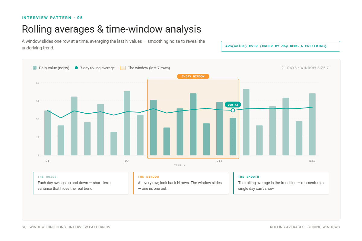
The window function used here is AVG(). Unlike in a simple average, a rolling or moving average doesn’t take into account all data points, but only a specified number of the preceding and/or following data points. Using preceding data points is more common. A centered moving average – the one that uses the current and the following rows – is less common, as those following rows might not exist yet; moving averages are typically used on live or recent data.
You could calculate the 3-day, 7-day, 30-day, 12-month averages, or whatever variation you desire.
For example, a 7-day rolling average includes the 6 previous days + the current day = 7 days. You calculate like that for each day. As you go, the size of the calculation window stays the same (7 days); it just moves day by day.
We’re Going Advanced: The Frame Clause in Window Functions
To calculate rolling averages and perform a time window analysis in window functions, you need to define the frame clause.
The generic syntax is given below.
<window_function>() OVER (
    [PARTITION BY column_name]
    [ORDER BY column_name]
    [ROWS | RANGE BETWEEN <frame_start> AND <frame_end>]
)
Here are the components of the frame clause.
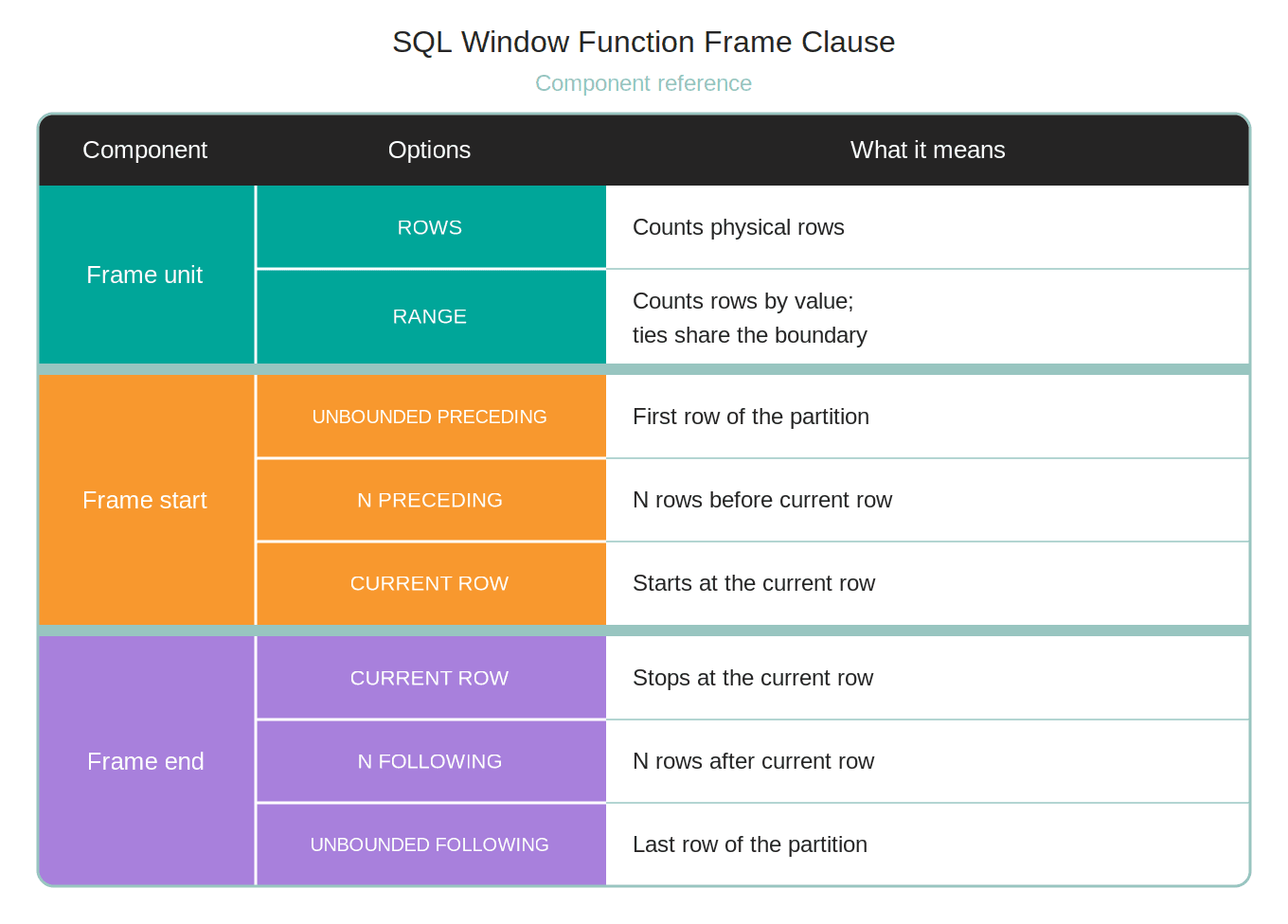
All these components can be combined in many different ways, which, in turn, results in different frame definitions. Here are the most common combinations.
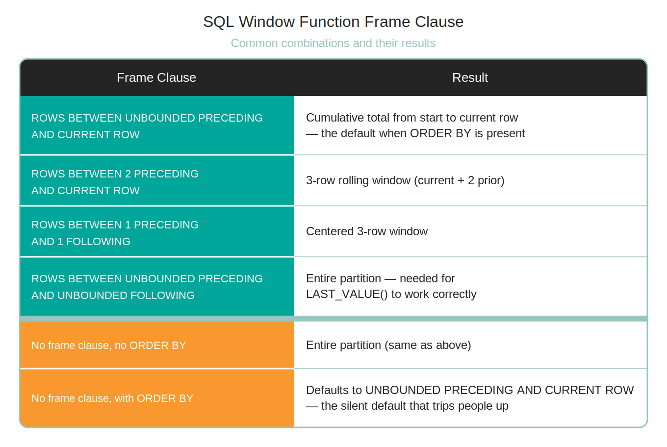
Now, let’s demonstrate this by solving one of the Amazon SQL interview questions.
Revenue Over Time
Last Updated: December 2020
Find the 3-month rolling average of total revenue from purchases given a table with users, their purchase amount, and date purchased. Do not include returns which are represented by negative purchase values. Output the year-month (YYYY-MM) and 3-month rolling average of revenue, sorted from earliest month to latest month.
A 3-month rolling average is defined by calculating the average total revenue from all user purchases for the current month and previous two months. The first two months will not be a true 3-month rolling average since we are not given data from last year. Assume each month has at least one purchase.
We have to calculate a 3-month rolling average of the revenue from purchases. The negative purchase values – i.e., the returns – shouldn’t be included in the calculation. The output should show YYYY-MM and the 3-month rolling average, sorted from the earliest to the latest month.
Dataset
There’s one table named amazon_purchases.
Solution
Let me first explain the subquery, then we’ll finish it off with the rolling average calculation.
1. Purchase sum by month
The subquery’s purpose is to sum all the purchases by month. We do that by using TO_CHAR to convert the created_at column to the YYYY-MM format, then applying SUM() to calculate monthly revenue.
The output is grouped by and sorted by month.
SELECT TO_CHAR(created_at::DATE, 'YYYY-MM') AS month,
       SUM(purchase_amt) AS monthly_revenue
FROM amazon_purchases
WHERE purchase_amt>0
GROUP BY TO_CHAR(created_at::DATE, 'YYYY-MM')
ORDER BY TO_CHAR(created_at::DATE, 'YYYY-MM')
Here’s its output.
| month | monthly_revenue |
|---|---|
| 2020-01 | 26292 |
| 2020-02 | 20695 |
| 2020-03 | 29620 |
| 2020-04 | 21933 |
| 2020-05 | 24700 |
| 2020-06 | 27687 |
| 2020-07 | 25309 |
| 2020-08 | 23496 |
| 2020-09 | 24827 |
| 2020-10 | 15310 |
2. Calculate the moving average
Now, we embed it into the outer query. The outer query calculates the moving average on the data provided by the subquery. The window function used is – expectedly – AVG(), with the window defined as ROWS BETWEEN 2 PRECEDING AND CURRENT ROW. This window definition means that the current row and the two before it are included in the calculation. Each row is one month; in other words, we calculate the moving average on the current and the two previous months.
Of course, the calculation has to run from the earliest to the latest month to make sense, so we sort the data in the window by month in ascending order in the OVER() clause.
Interview Pattern #6: Retention, Reactivation, and Session Patterns
This is probably the hardest pattern. Not because of any especially difficult window functions, but because it requires chaining multiple window functions.
This pattern encompasses three distinct problem types.
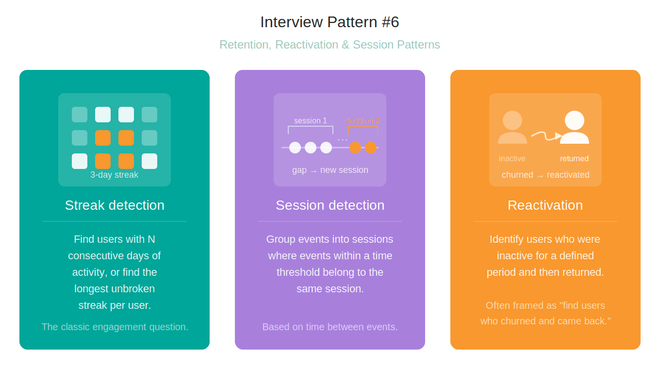
All three are instances of the classic islands-and-gaps problem.
Streak and session detection identify the periods of consecutive activity, i.e., the islands.
Reactivation focuses on gaps, i.e., detecting when a user’s silence exceeds a threshold before a new island begins.
This technique works in three steps.
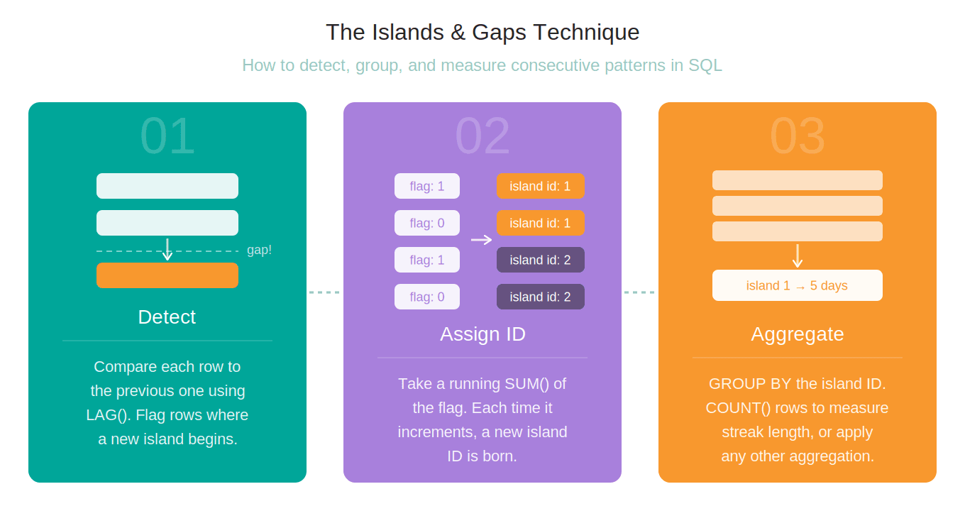
Let’s now apply this technique to an actual business problem.
Here’s an interview question from LinkedIn and Meta SQL interview questions.
User Streaks
Last Updated: October 2022
Provided a table with user ID and the dates they visited the platform, find the top 3 users with the longest continuous streak of visiting the platform up to August 10, 2022. Output the user ID and the length of the streak.
In case of a tie, display all users with the top three longest streak lengths.
We need to find the top three users with the longest platform visit streaks up to 10 August 2022. The output must show the user ID and the streak length in days.
Dataset
We’ll use the user_streaks table.
Solution
The solution chains several CTEs.
1. unique_visits CTE: Uses DISTINCT to find unique daily visits per user up to '2022-08-10'.
WITH unique_visits AS (
    SELECT DISTINCT user_id,
                    date_visited
    FROM user_streaks
    WHERE date_visited <= DATE '2022-08-10'
),
2. streak_flags CTE: In this CTE, we reference the previous CTE and use CASE WHEN to mark the new streak with 1. We calculate it by first using LAG() to access the date of the previous visit, then subtracting that date from the current session date. If the difference is 1 – one day – that’s a continuation of the streak, so we mark it as 0. Otherwise, it’s marked as 1.
streak_flags AS (
    SELECT *,
           CASE
               WHEN date_visited - LAG(date_visited) OVER (PARTITION BY user_id ORDER BY date_visited) = 1
               THEN 0
               ELSE 1
           END AS new_streak
    FROM unique_visits
),
3. streak_ids CTE: Here, we use another window function, namely SUM(), to calculate the cumulative sum of the streaks by user. The cumulative sum becomes a streak ID, assigned to each user’s date of visit. That way, we can identify the number of streaks and the number of visits within each streak.
streak_ids AS (
    SELECT *,
           SUM(new_streak) OVER (PARTITION BY user_id ORDER BY date_visited) AS streak_id
    FROM streak_flags
),
4. streak_lengths CTE: Now, we use the info from the previous CTE to COUNT(*) each user’s each streak’s length.
streak_lengths AS (
    SELECT user_id,
           streak_id,
           COUNT(*) AS streak_length
    FROM streak_ids
    GROUP BY user_id, streak_id
),
5. longest_per_user CTE: As a next step, we use MAX() to find the longest streak per user.
longest_per_user AS (
    SELECT user_id,
           MAX(streak_length) AS streak_length
    FROM streak_lengths
    GROUP BY user_id
),
6. ranked_lengths CTE: Now, we use DENSE_RANK() to rank each user’s streaks by their length, from the longest to shortest.
ranked_lengths AS (
    SELECT DISTINCT streak_length,
           DENSE_RANK() OVER (ORDER BY streak_length DESC) AS len_rank
    FROM longest_per_user
),
7. top_lengths CTE: In this final CTE, we simply keep only the three top longest streaks.
top_lengths AS (
    SELECT streak_length
    FROM ranked_lengths
    WHERE len_rank <= 3
)
Now, in the final step, everything comes together. We join the longest_per_user and top_lengths CTEs to connect the three longest streaks to their users, and show it as the output. Here’s the complete code.
Why the Interviewers Love This Pattern
To apply this pattern, you first need to recognize that the problem can’t be solved in one pass. That’s already a plus in the interviewer's notebook. Then, you demonstrate thinking in layers, as I showed you above: detecting, grouping, counting, ranking – each CTE has a clear, distinct purpose.
That way of thinking is what distinguishes candidates who understand data (and the problem) from those who just know syntax.
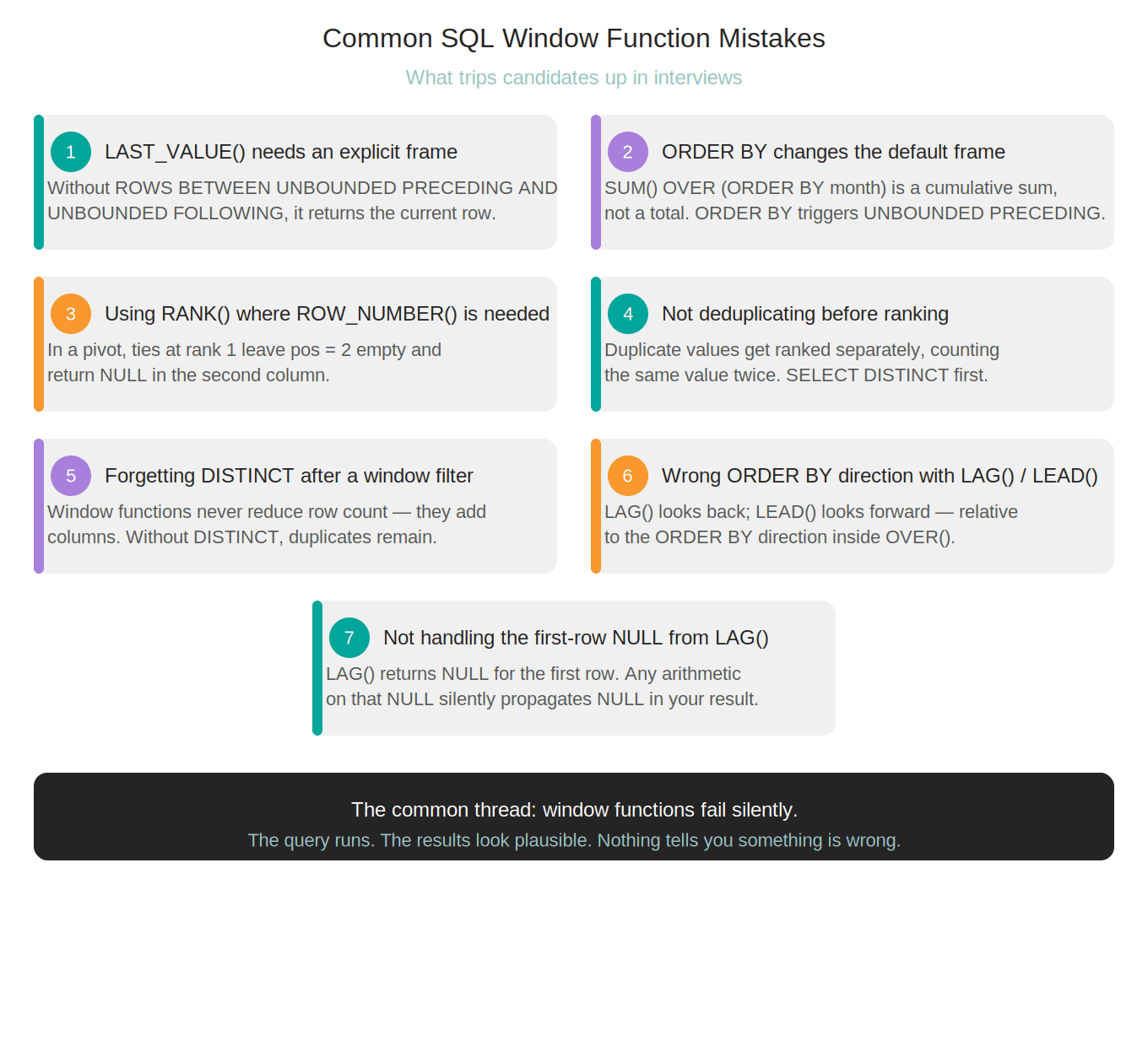
Common SQL Window Function Mistakes in Interviews
There are several typical window function mistakes candidates make in interviews. Often, these mistakes are silent: the query runs, it returns results, but nothing tells you the result is wrong.
Practice SQL Window Function Interview Questions
The time has come for you to stop reading and start actively practicing what this article has taught you. Here are several hand-picked StrataScratch questions for each window function pattern.
1. Practice: Finding the Latest Row per User
Question #1: Finding Updated Records
Finding Updated Records
Last Updated: November 2020
We have a table with employees and their salaries; however, some of the records are old and contain outdated salary information. Since there is no timestamp, assume salary is non-decreasing over time. You can consider the current salary for an employee is the largest salary value among their records. If multiple records share the same maximum salary, return any one of them. Output their id, first name, last name, department ID, and current salary. Order your list by employee ID in ascending order.
Dataset
Solution
Write, run, and check your solution in the code editor.
Question #2: Streamer Sessions by Initial Viewers
Streamer Sessions by Initial Viewers
Last Updated: January 2021
Return the number of streamer sessions for each user whose very first session was as a viewer.
Include the user ID and count of streamer sessions for users whose earliest session (by session_start) was a 'viewer' session, regardless of whether they ever had a streamer session later. Sort the results by streamer session count in descending order, then by user ID in ascending order.
Dataset
Solution
Write, run, and check your solution in the code editor.
Question #3: Highest Salary in the Department
Highest Salary In Department
Last Updated: April 2019
A business wants to identify its highest-paid employee in each department for compensation benchmarking and review. Find the employee with the highest salary in each department.
Output the department name, the employee's first name and their salary. If multiple employees share the highest salary in a department, return all of them.
Dataset
Solution
Write, run, and check your solution in the code editor.
2. Practice: Ranking Customers, Products, or Events
Question #1: Ranking Most Active Guests
Ranking Most Active Guests
Identify the most engaged guests by ranking them according to their overall messaging activity. The most active guest, meaning the one who has exchanged the most messages with hosts, should have the highest rank. If two or more guests have the same number of messages, they should have the same rank. Importantly, the ranking shouldn't skip any numbers, even if many guests share the same rank. Present your results in a clear format, showing the rank, guest identifier, and total number of messages for each guest, ordered from the most to least active.
Dataset
Solution
Write, run, and check your solution in the code editor.
Question #2: Best Selling Item
Best Selling Item
Last Updated: July 2020
Find the best-selling item for each month (no need to separate months by year). The best-selling item is determined by the highest total sales amount, calculated as: total_paid = unitprice * quantity. A negative quantity indicates a return or cancellation (the invoice number begins with 'C'. To calculate sales, ignore returns and cancellations. Output the month, description of the item, and the total amount paid.
Dataset
Solution
Write, run, and check your solution in the code editor.
Question #3: Rank Variance per Country
Rank Variance Per Country
Last Updated: February 2021
Compare the total number of comments made by users in each country during December 2019 and January 2020.
For each month, rank countries by their total number of comments in descending order. Countries with the same total should share the same rank, and the next rank should increase by one (without skipping numbers).
Return the names of the countries whose rank improved from December to January (that is, their rank number became smaller).
Dataset
Solution
Write, run, and check your solution in the code editor.
3. Practice: Calculating Running Totals & Cumulative Metrics
Question #1: Maximum Number of Employees Reached
Maximum Number of Employees Reached
Last Updated: June 2021
Write a query that returns every employee that has ever worked for the company. For each employee, calculate the greatest number of employees that worked for the company during their tenure and the first date that number was reached. The termination date of an employee should not be counted as a working day.
Your output should have the employee ID, greatest number of employees that worked for the company during the employee's tenure, and first date that number was reached.
Dataset
Solution
Write, run, and check your solution in the code editor.
Question #2: Customer Tracking
Customer Tracking
Last Updated: October 2022
Given users' session logs, calculate how many hours each user was active in total across all recorded sessions.
Note: The session starts when state=1 and ends when state=0.
Dataset
Solution
Write, run, and check your solution in the code editor.
4. Practice: Comparing Current Row to Previous or Next Row
Question #1: Monthly Percentage Difference
Monthly Percentage Difference
Last Updated: December 2020
Given a table of purchases by date, calculate the month-over-month percentage change in revenue. The output should include the year-month date (YYYY-MM) and percentage change, rounded to the 2nd decimal point, and sorted from the beginning of the year to the end of the year. The percentage change column will be populated from the 2nd month forward and can be calculated as ((this month's revenue - last month's revenue) / last month's revenue)*100.
Dataset
Solution
Write, run, and check your solution in the code editor.
Question #2: Growth of Airbnb
Growth of Airbnb
Last Updated: February 2018
Calculate Airbnb's annual growth rate using the number of registered hosts as the key metric. The growth rate is determined by:
Growth Rate = ((Number of hosts registered in the current year - number of hosts registered in the previous year) / number of hosts registered in the previous year) * 100
Output the year, number of hosts in the current year, number of hosts in the previous year, and the growth rate. Round the growth rate to the nearest percent. Sort the results in ascending order by year.
Assume that the dataset consists only of unique hosts, meaning there are no duplicate hosts listed.
Dataset
Solution
Write, run, and check your solution in the code editor.
Question #3: Finding User Purchases
Finding User Purchases
Last Updated: December 2020
Identify returning active users by finding users who made a second purchase within 1 to 7 days after their first purchase. Ignore same-day purchases. Output a list of these user_ids.
Dataset
Solution
Write, run, and check your solution in the code editor.
5. Practice: Rolling Averages and Time-Window Analysis
Question #1: Distance per Dollar
Distance Per Dollar
Last Updated: November 2020
You’re given a dataset of Uber rides with the traveling distance (distance_to_travel) and cost (monetary_cost) for each ride. First, find the difference between the distance-per-dollar for each ride and the monthly distance-per-dollar for that year-month.
Distance-per-dollar for each ride is defined as the distance traveled divided by the cost of the ride. Monthly distance-per-dollar is defined as the total distance traveled in that month divided by the total cost for that month.
Use the calculated difference on each date to calculate absolute average difference in distance-per-dollar metric on monthly basis (year-month).
The output should include the year-month (YYYY-MM) and the absolute average difference in distance-per-dollar (Absolute value to be rounded to the 2nd decimal).
You should also count both success and failed request_status as the distance and cost values are populated for all ride requests. Also, assume that all dates are unique in the dataset. Order your results by earliest request date first.
Dataset
Solution
Write, run, and check your solution in the code editor.
Question #2: Product Engagement Momentum Shifts
Product Engagement Momentum Shifts
Last Updated: September 2024
Identify all products that experienced a turnaround in user engagement: at least 3 consecutive months of declining monthly active users followed by at least 3 consecutive months of growth.
For each product that matches this pattern, return the product name, the month when the decline started, the month when growth resumed, and the growth ratio from the lowest point to the most recent peak, calculated as: (peak_users - lowest_users) / lowest_users.
Dataset
Solution
Write, run, and check your solution in the code editor.
Question #3: Search Click Success Rate by User Segment
Search Click Success Rate by User Segment
Last Updated: October 2025
Calculate the search success rate for new users versus existing users. A successful search is one where the first click event occurs within 30 seconds of the search event.
Group all users into two segments:
• new (registered within the last 30 days covered by the dataset — that is, on or after 30 days before the most recent date in the dataset)
• existing (registered earlier).
Return one row per user segment with total searches, successful searches, and success rate.
Dataset
Solution
Write, run, and check your solution in the code editor.
6. Practice: Retention, Reactivation, and Session Patterns
Question #1: Consecutive Days
Consecutive Days
Last Updated: July 2021
Find all the users who were active for 3 consecutive days or more.
Dataset
Solution
Write, run, and check your solution in the code editor.
Question #2: Users by Average Session Time
Users By Average Session Time
Last Updated: July 2021
Calculate each user's average session time, where a session is defined as the time difference between a page_load and a page_exit. Assume each user has only one session per day. If there are multiple page_load or page_exit events on the same day, use only the latest page_load and the earliest page_exit. Only consider sessions where the page_load occurs before the page_exit on the same day. Output the user_id and their average session time.
Dataset
Solution
Write, run, and check your solution in the code editor.
Question #3: First Day Retention Rate
First Day Retention Rate
Last Updated: February 2022
Calculate the first-day retention rate of a group of video game players. The first-day retention occurs when a player logs in 1 day after their first-ever log-in. Return the proportion of players who meet this definition divided by the total number of players.
Dataset
Solution
Write, run, and check your solution in the code editor.
Final Takeaway
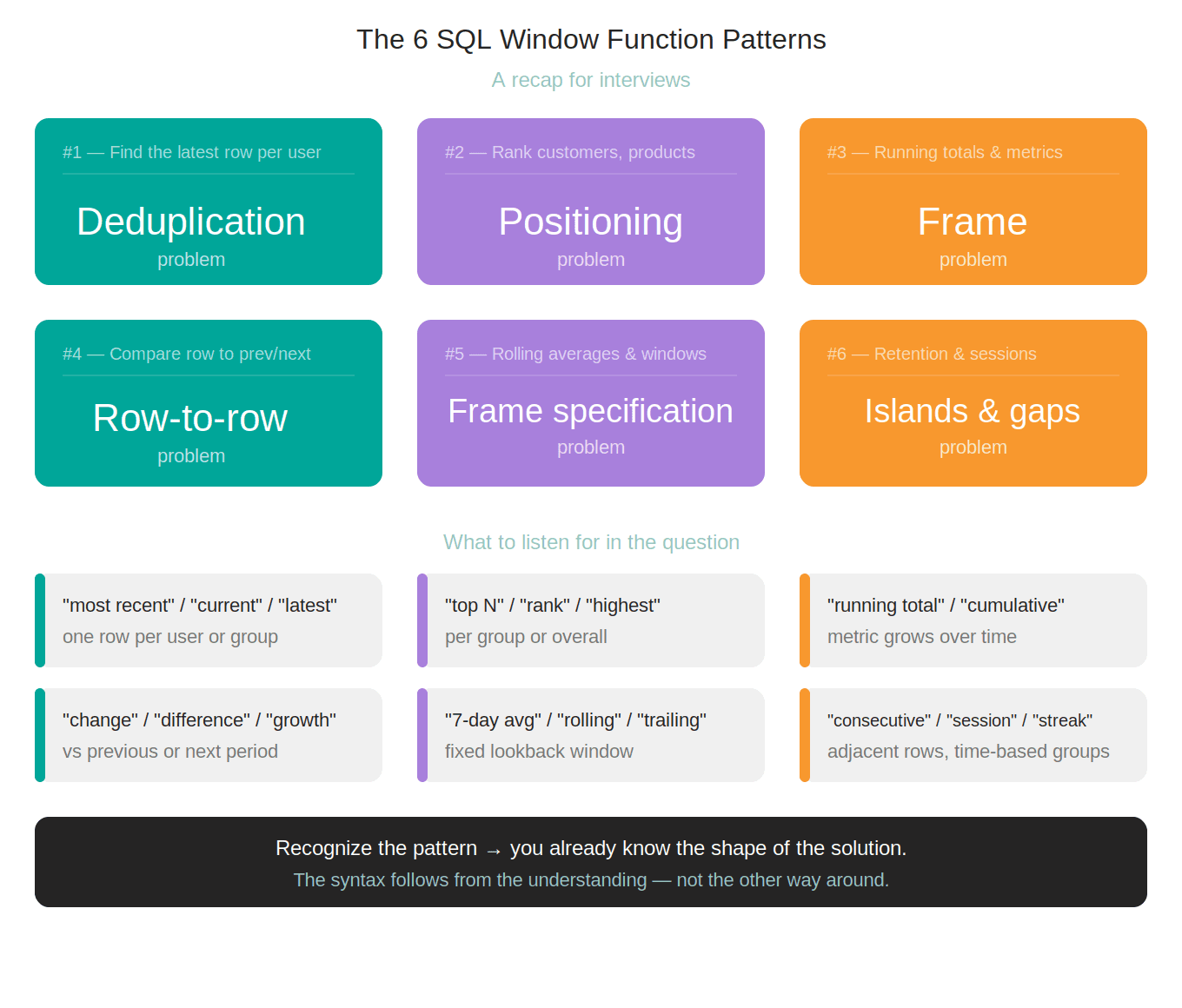
This guide gave you a framework for recognizing which problem calls for which window function. I’ve shown you six patterns that cover the vast majority of SQL interview questions where you’ll encounter window functions.
Let’s recap them.
The best way to build a real understanding of these patterns is to work through the questions. Write the code yourself, get it wrong, understand why, and fix it. This is the only way to stop thinking about the window function syntax and start thinking about business problem-solving. It sets you on the path to an interview and job success.
FAQs
1. What is the difference between GROUP BY and a window function?
GROUP BY collapses individual rows and returns one row per group. Window functions don’t do that; they perform a calculation along the individual rows, show the result, and keep the individual rows.
2. Which SQL window functions are most common in interviews?
ROW_NUMBER(): Probably the most common one. Used in deduplication, finding the first or last row per group, and pivoting ranked results into columns.RANK()&DENSE_RANK(): They show up in top-N problems.LAG()&LEAD(): We use them for row-to-row comparisons, such as month-over-month change, time between events, and comparing a value to the previous period.SUM() OVER,AVG() OVER,COUNT() OVER: These are aggregate window functions. Used to calculate group-level metrics at the row level, most commonly running totals and moving averages.FIRST_VALUE()&LAST_VALUE(): Used to pull a value from the first or the last row of a partition. They are a common alternative toROW_NUMBER()when you only need one column, not the whole row
3. When should I use ROW_NUMBER() vs RANK()?
The difference only matters when there are ties, i.e., two or more rows with the same value in the ORDER BY clause in OVER().
ROW_NUMBER() always assigns a unique integer to every row. So, it ignores ties and breaks them nondeterministically. You should use this window function whenever the logic requires WHERE rank = 1, i.e., returning a single row. Common examples are deduplication and pivoting positions into columns.
RANK() should be used when tied rows should share a position and all should appear in the results, because this function assigns the same rank to tied rows, then skips the next rank.
DENSE_RANK() is a third option, which assigns the same rank to tied rows – just like RANK() – but without skipping the next rank. Use it when you want the Nth-highest value always to be ranked as N, regardless of how many rows share rank N-1.
4. How do I calculate a running total in SQL?
By using SUM() as a window function with ORDER BY inside OVER().
SELECT date,
       revenue,
       SUM(revenue) OVER (ORDER BY date) AS running_total
FROM daily_revenue;
Such use of the ORDER BY clause activates a default frame of ROWS BETWEEN UNBOUNDED PRECEDING AND CURRENT ROW. This means the sum includes all rows from the beginning of the result up to and including the current row. This is a textbook definition of a running or cumulative total.
You can, of course, do the same for each group by using the PARTITION BY clause. In the example below, running totals are calculated per user.
SELECT date,
       revenue,
       SUM(revenue) OVER (PARTITION BY user_id ORDER BY date)
FROM daily_revenue;
Note that ORDER BY in OVER() is what makes the SUM() window function calculate cumulatives. If you use the SUM() OVER() version, that gives the same grand total in every row.
5. What do LAG() and LEAD() do?
LAG() lets you access the value from the previous row on N rows, ordered by the ORDER BY clause in OVER().
LEAD() does the same, only for the next row on N rows.
6. How do rolling windows work in SQL?
Rolling windows within window functions limit the calculation to a fixed number of preceding and or following rows, rather than all rows from the start.
The window frame clause has two parts. The first part is the unit, i.e., ROWS or RANGE . ROWS counts physical rows, RANGE determines the included number of rows by value.
The second part of the window frame clause is the bounds BETWEEN … AND …, which define how far the window extends in each direction from the current window. Each bound endpoint – a start or an end – can be one of these five values:
UNBOUNDED PRECEDING– the first row of the partitionN PRECEDING– N rows before the current rowCURRENT ROW– the current row itselfN FOLLOWING– N rows after the current rowUNBOUNDED FOLLOWING– the last row of the partition
For example, a rolling window defined as ROWS BETWEEN 2 PRECEDING AND CURRENT ROW means the window function performs a calculation on 2 rows preceding the current row and the current row, which makes it a 3-row rolling window.
Share