SQL Execution Order Explained With Real Query Examples

Categories:
 Written by:
Sara Nobrega
SQL execution order decides how queries actually run. Learn why FROM comes first, how aliases fail in WHERE, and when to use HAVING, with real examples.
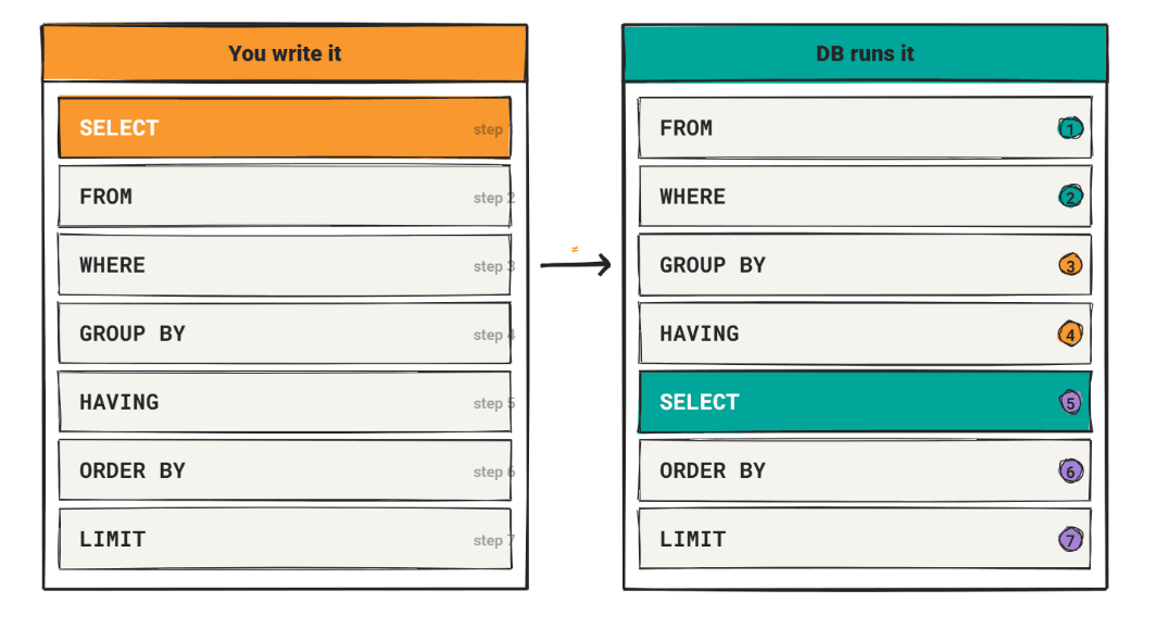
A query reads top to bottom, starting with SELECT. The database engine does not run it that way. It starts with FROM, builds the rows, filters them, groups them, and only then evaluates SELECT. Once you know that order, a whole class of confusing errors stops being confusing: why an alias from SELECT fails in WHERE, why a window function cannot sit in WHERE, why an aggregate filter has to go in HAVING.
In this guide, we walk through the logical processing order one step at a time, then prove each rule against real StrataScratch interview questions. Every query here is a live PostgreSQL [LINK] solution you can run in the editor.
What Is SQL Execution Order?
SQL execution order is the sequence the database follows when it evaluates the clauses of a query. SQL is a declarative language: you describe the result you want, and the engine decides how to produce it. The clause you write first is rarely the clause that runs first.
There are two orders worth separating. The logical order is the conceptual sequence the standard defines, and it is what we cover here. The physical order is what the query optimizer actually does at runtime, which can reorder or merge steps for speed as long as the result matches the logical order. For writing correct queries and reading them in interviews, the logical order is what matters.
SQL Logical Query Processing Order
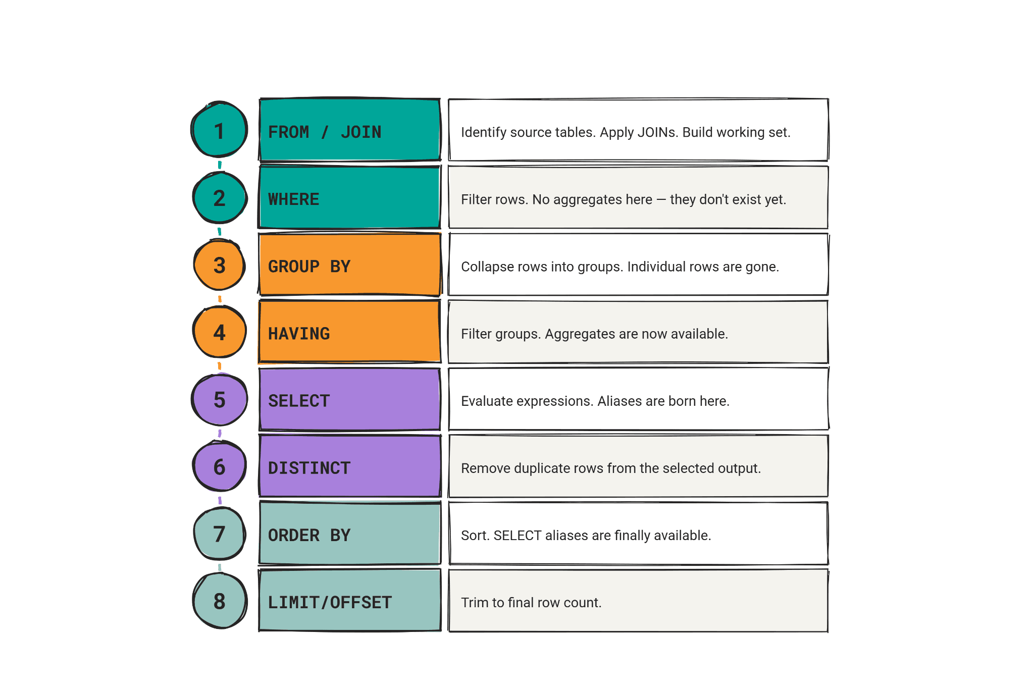
The logical SQL execution order has nine steps. Each step takes the output of the previous one as its input, which is why a clause can only reference what earlier steps have already produced.
Step 1: FROM
FROM runs first. It identifies the source tables and pulls in the starting set of rows. Everything downstream operates on this set, so the row count after FROM is the baseline you compare every later step against.
Step 2: JOIN
Joins combine the source tables into one working set. A join can multiply rows: if one row on the left matches three rows on the right, you get three output rows. This happens before any filtering or grouping, so the grain you start grouping with is the grain the join produced, not the grain of either original table.
Step 3: WHERE
WHERE filters individual rows, and it runs before any grouping or aggregation. At this point, there are no groups or aggregate values yet, so WHERE can only test column values on single rows. This is the reason why an aggregate condition like COUNT(*) >= 5 cannot live in WHERE.
Step 4: GROUP BY
GROUP BY collapses the filtered rows into groups, one group per distinct combination of the grouping columns. After this step, the working set is one row per group, and aggregate functions like SUM, COUNT, and AVG are computed over the rows within each group.
Step 5: HAVING
HAVING filters groups, and it runs after aggregation. Because the aggregate values now exist, HAVING is where group-level conditions belong, such as keeping only departments with five or more employees.
Step 6: SELECT
SELECT is written first but runs sixth. This is where output columns are computed, expressions are evaluated, and aliases are assigned. Window functions are also evaluated around this step, after grouping. Because aliases are created here, no earlier clause (WHERE, GROUP BY, HAVING) can see them.
Step 7: DISTINCT
DISTINCT removes duplicate rows from the result of SELECT. It runs after the output columns are created, so it deduplicates the projected rows rather than the source rows.
Step 8: ORDER BY
ORDER BY sorts the final result. It runs late enough to reference SELECT aliases, which is why ordering by a computed alias like apartment_count works, while filtering on it in WHERE does not.
Step 9: LIMIT / TOP / FETCH
LIMIT (PostgreSQL and MySQL [LINK]), TOP (SQL Server [LINK]), and FETCH FIRST (Oracle [LINK]) all run last. They slice the sorted result down to a fixed number of rows. Because this is the final step, the ORDER BY sort is already complete by the time the slice occurs.
SQL Execution Order Flow Diagram
Here is the full SQL execution order as a single sequence. Each clause feeds the next:
FROMandJOIN: build and combine the source rowsWHERE: filter individual rowsGROUP BY: collapse rows into groupsHAVING: filter groups using aggregatesSELECT: compute output columns, aliases, and window functionsDISTINCT: remove duplicate output rowsORDER BY: sort the resultLIMIT/TOP/FETCH: cut the result to a fixed number of rows
The written order you type is almost the reverse of the run order at the top: SELECT is line one but step five.
Why SQL Executes Differently Than It Is Written
The gap between written order and execution order exists because SQL is declarative. You state the shape of the answer, and the engine picks an evaluation order that can produce it. The logical order puts data assembly first (FROM, JOIN), narrowing second (WHERE), summarizing third (GROUP BY, HAVING), and presentation last (SELECT, ORDER BY, LIMIT).
This sequence explains the rules that trip people up:
- An alias defined in
SELECTis invisible toWHERE,GROUP BY, andHAVING, because all of those run beforeSELECT. - An aggregate condition belongs in
HAVING, notWHERE, because aggregates do not exist untilGROUP BYhas run. - A window function cannot be referenced in
WHEREof the same query, because window functions are evaluated aroundSELECT, well afterWHERE.
The examples below show each of these against a real query.
Real SQL Execution Order Examples
Example 1: Filtering Before Aggregation
The cleanest way to see SQL execution order in one query is a pipeline that filters rows, groups them, and then filters the groups. This question does all three.
Department Workforce Analysis
Last Updated: March 2025
The workforce planning team is analyzing department growth since the company's expansion, focusing on teams that have grown substantially.
For each department with 5 or more employees hired after 2020, return the name, headcount, total payroll, and average salary.
Data View
The techcorp_workforce table holds one row per employee, with their department, salary, and joining date. The task asks, for each department with five or more employees hired after 2020, for the department name, headcount, total payroll, and average salary.
Grain (what one output row means): one department that passes both the date filter and the headcount threshold.
Interview Framing
When we see this asked in interviews, the follow-up is almost always "where does each filter go, and why?" The date condition is row-level, so it runs in WHERE before grouping. The headcount condition is group-level, so it runs in HAVING after grouping. A candidate who can say that out loud, in execution order, is showing they understand the pipeline rather than guessing.
Common Mistakes
The frequent mistake is trying to filter the headcount in WHERE: writing WHERE COUNT(*) >= 5. That fails, because WHERE runs at step 3 and COUNT(*) does not exist until GROUP BY runs at step 4. The headcount filter has to move to HAVING. A second mistake is assuming the headcount alias from SELECT can be reused in WHERE or HAVING. It cannot, because SELECT runs after both.
Solution
The WHERE joining_date > '2020-12-31' shrinks the rows first, so only post-2020 hires reach the grouping step. GROUP BY department then forms one row per department, and HAVING COUNT(*) >= 5 drops the small teams.
Output
| department | headcount | total_payroll | avg_salary |
|---|---|---|---|
| Finance | 7 | 547000 | 78142.86 |
| Sales | 7 | 484000 | 69142.86 |
| Engineering | 8 | 769000 | 96125 |
| HR | 8 | 595500 | 74437.5 |
| Admin | 7 | 475500 | 67928.57 |
Example 2: HAVING vs WHERE
The previous example mixed a row filter and a group filter. This one strips the idea down to its smallest form: a single group-level condition with no row filter at all.
Departments With 5 Employees
Last Updated: May 2019
Find departments with at more than or equal 5 employees.
Data View
The employee table holds one row per employee, with department, salary, and identifying columns. The task is to find departments with five or more employees.
Grain (what one output row means): one department that has at least five employees.
Trade-offs
The condition we care about, "at least five employees," is a count, and a count only exists after grouping. So the only correct home for it is HAVING. There is no row-level version of this filter, because no single row knows how many employees its department has. That is the decision rule: if the condition needs an aggregate, it goes in HAVING; if it only needs values from one row, it goes in WHERE.
Solution
GROUP BY department forms the groups, then HAVING COUNT(DISTINCT id) >= 5 keeps only the departments whose distinct employee count clears the threshold. We use COUNT(DISTINCT id) rather than COUNT(*) to count each employee once even if a row appears more than once.
Output
| department |
|---|
| Sales |
Example 3: Why Window Functions Cannot Be Used in WHERE
Window functions are evaluated around SELECT, after WHERE has already run. This question forces that point: you have to compute a rank and then filter on it, which means two passes.
Second Highest Salary
Last Updated: April 2019
Find the second highest salary of employees.
Data View
The employee table again holds one row per employee with a salary column. The task is to find the second highest salary.
Grain (what one output row means): one salary value, the one ranked second from the top.
Common Mistakes
The instinct is to rank and filter in the same query: ... DENSE_RANK() OVER (ORDER BY salary DESC) AS salary_rank ... WHERE salary_rank = 2. That errors. WHERE runs at step 3, and salary_rank is a window function evaluated around SELECT at step 6, so the column does not exist yet when WHERE looks for it. The fix is to compute the rank in a CTE (its own SELECT), then filter the rank in an outer query, where it now exists as a plain column.
Solution
1) Rank every salary in a CTE.
We compute DENSE_RANK() over salaries in descending order. This is the inner SELECT, so the rank becomes a real column once the CTE is materialized.
SELECT salary,
       DENSE_RANK() OVER (ORDER BY salary DESC) AS salary_rank
FROM employee;
2) Filter the rank in the outer query (final solution).
In the outer query, salary_rank is an ordinary column from the CTE, so WHERE salary_rank = 2 is legal. DISTINCT collapses ties so the second-highest salary appears once.
Output
| salary |
|---|
| 200000 |
Example 4: JOIN Duplication Before GROUP BY
Joins run at step 2, before grouping at step 4. That order is why a join can quietly inflate your counts unless you account for the rows it produces.
Number Of Units Per Nationality
Write a query that returns how many different apartment-type units (counted by distinct unit_id) are owned by people under 30, grouped by their nationality. Sort the results by the number of apartments in descending order.
Data View
The airbnb_units table holds one row per unit, with unit_id, unit_type, and the owning host_id. The airbnb_hosts table holds one row per host, with age and nationality. The task is to count distinct apartment-type units owned by hosts under 30, grouped by nationality, sorted by count in descending order.
Grain (what one output row means): one nationality, with the number of distinct apartment units owned by hosts under 30.
Common Mistakes
After the join runs, the working set is at unit-and-host grain, and a plain COUNT(*) would count join rows rather than units. Using COUNT(DISTINCT unit_id) counts each unit once and guards against the duplication introduced by the join. A second point about order: apartment_count is an alias from SELECT, so ORDER BY apartment_count DESC works (step 8 runs after SELECT), but the same alias in WHERE would fail.
Validation
To confirm the grain, check the row count right after the join, then after GROUP BY. The post-join count tells you how much the join multiplied rows; the post-group count should equal the number of distinct nationalities that survive the age < 30 and unit_type = 'Apartment' filters.
Solution
Output
| nationality | apartment_count |
|---|---|
| USA | 2 |
Example 5: LIMIT in Action: Hour Of Highest Gas Expense
A clean way to see the last two steps work together is a top-one question solved with ORDER BY plus LIMIT, with no aggregation or window function involved.
Hour Of Highest Gas Expense
Find the hour of the single ride with the highest gasoline cost. Assume only one ride has this maximum, so exactly one hour qualifies.
Data View
The lyft_rides table contains one row per ride, with the ride hour, gasoline cost, travel distance, and weather. The task is to find the single hour with the highest gasoline cost.
Grain (what one output row means): one hour, the one with the largest gasoline_cost.
Why This Demonstrates Execution Order
ORDER BY gasoline_cost DESC runs at step 8 and sorts the entire result set from highest to lowest cost. Only then does LIMIT 1 run at step 9 and keep the top row. Drop the ORDER BY and LIMIT 1 returns an arbitrary hour, because there is nothing to slice against. The sort has to finish before the slice means anything.
In other dialects, the final step changes name but not position: SQL Server writes SELECT TOP 1 ... ORDER BY ..., and Oracle writes ... ORDER BY ... FETCH FIRST 1 ROWS ONLY. The ordering still happens first.
Solution
Output
| hour |
|---|
| 10 |
Common SQL Execution Order Mistakes
Most SQL execution order bugs come from putting a clause in the wrong place relative to the step that produces what it needs. Here are the ones we see most often.
Filtering Aggregated Columns in WHERE
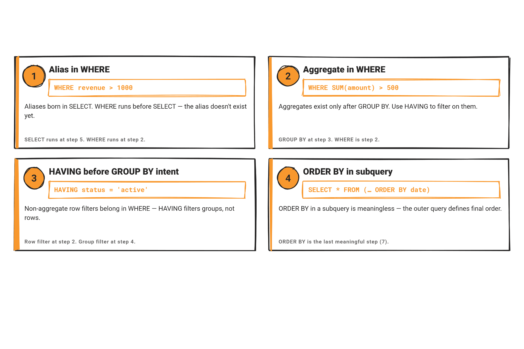
Writing WHERE COUNT(*) >= 5 is the classic version. WHERE runs at step 3, before GROUP BY at step 4, so no aggregate value exists yet. The filter belongs in HAVING. Example 1 (techcorp_workforce) and Example 2 (employee) both show the correct placement: row filters in WHERE, aggregate filters in HAVING.
Using SELECT Aliases Too Early
An alias defined in SELECT does not exist for WHERE, GROUP BY, or HAVING, because SELECT runs at step 6 after all of them. In Example 1, the headcount alias cannot be reused in HAVING; you have to repeat COUNT(*). The one place an alias is visible is ORDER BY, which runs at step 8, as Example 4 shows with ORDER BY apartment_count DESC.
Misplacing Window Functions
A window function evaluated in SELECT cannot be filtered in the same query, because WHERE already ran. The fix is to compute the window in a CTE or subquery and filter it one level up. This capstone question stacks that idea on top of row filtering, grouping, and an aggregate inside the window itself.
Best Selling Item
Last Updated: July 2020
Find the best-selling item for each month (no need to separate months by year). The best-selling item is determined by the highest total sales amount, calculated as: total_paid = unitprice * quantity. A negative quantity indicates a return or cancellation (the invoice number begins with 'C'. To calculate sales, ignore returns and cancellations. Output the month, description of the item, and the total amount paid.
Data View
The online_retail table holds one row per line item on an invoice, with invoicedate, description, unitprice, and quantity. The task is to find the best-selling item per month by total amount paid, ignoring returns (rows where quantity is negative).
Grain (what one output row means): one month, with the single highest-selling item description and its total paid.
Why This Stacks Every Rule
Reading the inner query in execution order: WHERE quantity > 0 filters rows at step 3, GROUP BY aggregates at step 4, and the RANK() window function is evaluated at step 6 over the already-aggregated result, ordering by SUM(unitprice * quantity). The rank cannot be filtered inside that same SELECT, so the whole thing sits in a CTE, and the outer query applies WHERE rnk = 1. Trying WHERE rnk = 1 in the inner query would error for the same reason as Example 3.
Solution
1) Aggregate per month and item, and rank inside a CTE.
We sum sales per month and description, then rank those sums within each month. The window orders by an aggregate, which is allowed because window functions run after GROUP BY.
SELECT
    date_part('month', invoicedate) AS month,
    description,
    SUM(unitprice * quantity) AS total_paid,
    RANK() OVER (
        PARTITION BY date_part('month', invoicedate)
        ORDER BY SUM(unitprice * quantity) DESC
    ) AS rnk
FROM online_retail
WHERE quantity > 0
GROUP BY date_part('month', invoicedate), description;
2) Keep the top-ranked item per month in the outer query (final solution).
Now rnk is a plain column, so WHERE rnk = 1 is legal.
Output
| month | description | total_paid |
|---|---|---|
| 1 | LUNCH BAG SPACEBOY DESIGN | 74.26 |
| 2 | REGENCY CAKESTAND 3 TIER | 38.25 |
| 3 | PAPER BUNTING WHITE LACE | 102 |
| 4 | SPACEBOY LUNCH BOX | 23.4 |
| 5 | PAPER BUNTING WHITE LACE | 51 |
| 6 | Dotcomgiftshop Gift Voucher £50.00 | 41.67 |
| 7 | PAPER BUNTING WHITE LACE | 56.1 |
| 8 | LUNCH BAG PINK POLKADOT | 16.5 |
| 9 | RED RETROSPOT PEG BAG | 34.72 |
| 10 | CHOCOLATE HOT WATER BOTTLE | 102 |
| 11 | RED WOOLLY HOTTIE WHITE HEART. | 228.25 |
| 12 | PAPER BUNTING RETROSPOT | 35.4 |
Unexpected Duplicates After JOIN
When you join through a bridge table, rows fan out before GROUP BY ever sees them. If you forget that, your sums double-count. This multi-table question makes the fan-out the whole point.
Risky Projects
Last Updated: November 2020
You are given a set of projects and employee data. Each project has a name, a budget, and a specific duration, while each employee has an annual salary and may be assigned to one or more projects for particular periods. The task is to identify which projects are overbudget. A project is considered overbudget if the prorated cost of all employees assigned to it exceeds the project’s budget.
To solve this, you must prorate each employee's annual salary based on the exact period they work on a given project, relative to a full year. For example, if an employee works on a six-month project, only half of their annual salary should be attributed to that project. Sum these prorated salary amounts for all employees assigned to a project and compare the total with the project’s budget.
Your output should be a list of overbudget projects, where each entry includes the project’s name, its budget, and the total prorated employee expenses for that project. The total expenses should be rounded up to the nearest dollar. Assume all years have 365 days and disregard leap years.
Data View
linkedin_projects holds one row per project with its budget and date range. linkedin_emp_projects is the bridge table linking employees to projects. linkedin_employees holds one row per employee with an annual salary. The task is to find projects whose prorated employee cost is over budget.
Grain (what one output row means): one over-budget project, with its budget and total prorated employee expense.
Common Mistakes
Joining through linkedin_emp_projects produces one row per employee-per-project, so the working set is at assignment grain, not project grain. GROUP BY collapses it back to one row per project, and only then does the prorated cost make sense to compare against the budget. The budget comparison is an aggregate (SUM(c.salary)), so it has to live in HAVING, not WHERE. Writing the comparison in WHERE fails because the sum does not exist before grouping.
Validation
Check the row count after both joins to see the fan-out, then confirm the final output is one row per project. If a project's expense looks too high, the usual cause is an extra join row inflating the SUM.
Solution
Output
| title | budget | prorated_employee_expense |
|---|---|---|
| Project1 | 29498 | 36293 |
| Project11 | 11705 | 31606 |
| Project12 | 10468 | 62843 |
| Project14 | 30014 | 36774 |
| Project16 | 19922 | 21875 |
| Project18 | 10302 | 46381 |
| Project2 | 32487 | 52870 |
| Project20 | 19497 | 55962 |
| Project21 | 24330 | 57310 |
| Project22 | 18590 | 20090 |
| Project24 | 11918 | 74665 |
| Project25 | 38909 | 57975 |
| Project26 | 36190 | 79368 |
| Project29 | 10935 | 48371 |
| Project30 | 24011 | 53106 |
| Project32 | 12356 | 66523 |
| Project33 | 30110 | 50034 |
| Project34 | 16344 | 23102 |
| Project35 | 23931 | 28652 |
| Project36 | 4676 | 25253 |
| Project37 | 8806 | 61949 |
| Project4 | 15776 | 30656 |
| Project42 | 24934 | 28301 |
| Project44 | 22885 | 49271 |
| Project46 | 9824 | 42314 |
| Project50 | 18915 | 23608 |
| Project6 | 41611 | 63230 |
| Project9 | 32341 | 44691 |
Confusing WHERE and HAVING
WHERE and HAVING are often confused. The rule from execution order is short: WHERE filters rows at step 3, before grouping; HAVING filters groups at step 5, after aggregation. If your condition references a single row's column, it goes in WHERE. If it references an aggregate, it goes in HAVING. Example 1 uses both in one query, which is the clearest way to keep them straight: the date filter in WHERE, the count filter in HAVING.
Misunderstanding DISTINCT and GROUP BY
DISTINCT and GROUP BY can both remove duplicates, but they enter at different steps. GROUP BY runs at step 4 and collapses rows into groups before SELECT. DISTINCT runs at step 7 and deduplicates the projected rows after SELECT. When there is no aggregate, they produce the same result, and this question is a good place to see why.
Matching Similar Hosts and Guests
Find matching hosts and guests pairs in a way that they are both of the same gender and nationality. Output the host id and the guest id of matched pair.
Data View
The airbnb_hosts table holds one row per host with gender and nationality. The airbnb_guests table holds one row per guest with the same attributes. The task is to find host-and-guest pairs that share both gender and nationality, and return the host ID and guest ID.
Grain (what one output row means): one unique host-and-guest pair that matches on gender and nationality.
Trade-offs
The join on (nationality, gender) can emit the same (host_id, guest_id) pair more than once, so the query uses SELECT DISTINCT to collapse duplicates at step 7. This rewrites one-for-one as GROUP BY h.host_id, g.guest_id with no aggregate selected. Both give the same rows here, because no aggregation is involved. The difference is when each one acts: GROUP BY collapses during grouping, DISTINCT collapses during the final projection. For pure deduplication of selected columns, DISTINCT reads more clearly; once you need an aggregate per group, GROUP BY is the only option.
Solution
Output
| host_id | guest_id |
|---|---|
| 0 | 9 |
| 1 | 5 |
| 2 | 1 |
| 3 | 7 |
| 4 | 0 |
| 5 | 2 |
| 6 | 4 |
| 7 | 10 |
| 8 | 3 |
| 9 | 8 |
| 10 | 6 |
| 11 | 11 |
How to Validate Queries Using SQL Execution Order
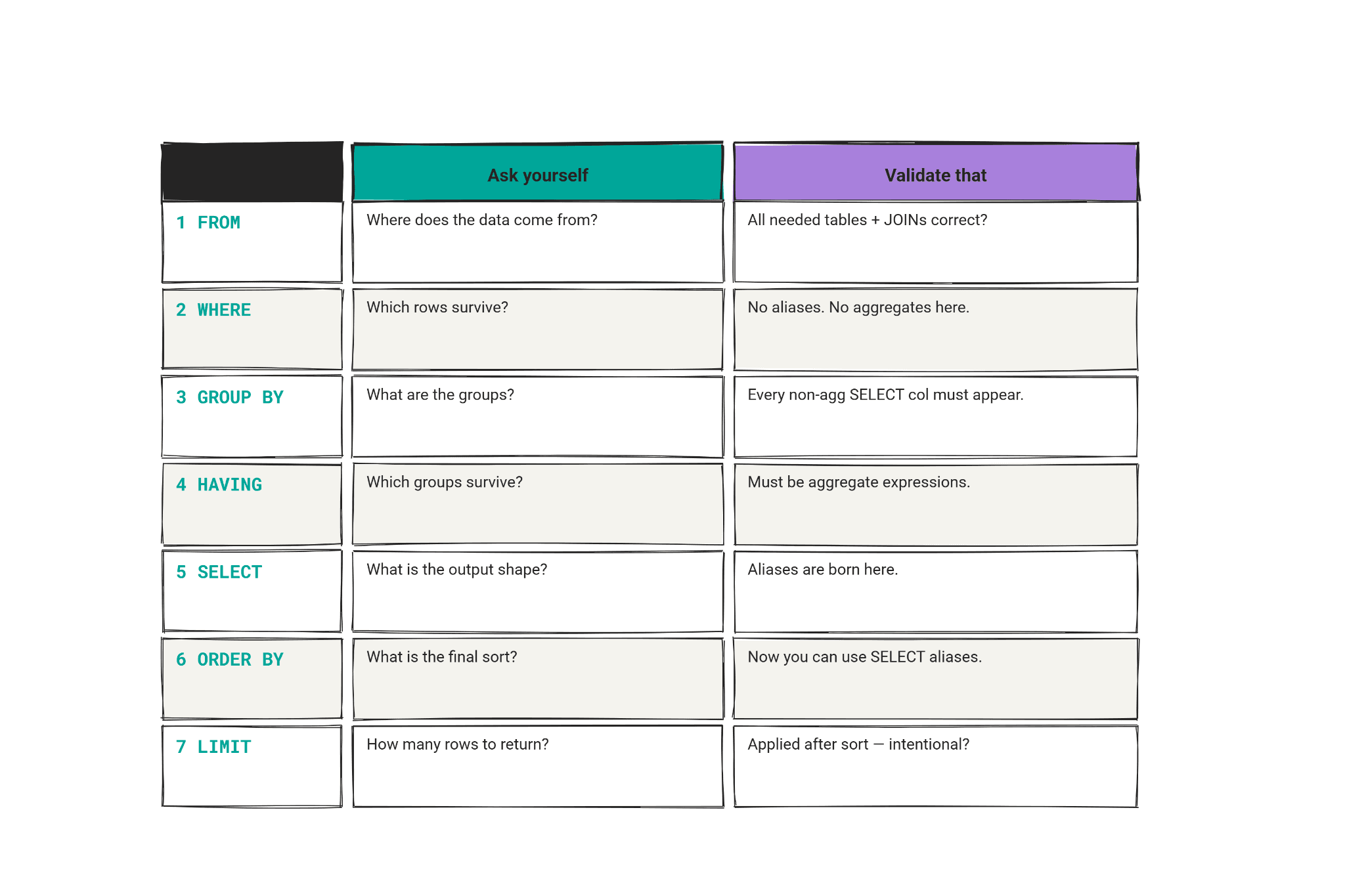
You can use the execution order as a checklist to confirm a query is correct, step by step. The idea is to inspect the working set after each step rather than only looking at the final output.
Check Row Counts After FROM and JOIN
Run the query up to the joins only, and count the rows. This tells you the grain you are actually working with before any filtering. In the linkedin_projects example, the count after both joins is at assignment grain, which is what makes the later GROUP BY necessary. A surprising row count here is the earliest sign a join is fanning out more than you expected.
Test WHERE Filters Separately
Run the WHERE clause on its own, without grouping, and confirm it keeps the rows you expect. In the techcorp_workforce example, checking WHERE joining_date > '2020-12-31' alone confirms only post-2020 hires survive before they reach GROUP BY. Isolating the filter separates a row-filtering bug from a grouping bug.
Verify Aggregation Grain Before GROUP BY
Before trusting any aggregate, confirm what one output row will mean. After GROUP BY department, you should have exactly one row per department. If you see more, a grouping column is too fine; if sums look doubled, a join upstream multiplied rows. The airbnb_units example is a good check: the output should be one row per nationality.
Validate GROUP BY Results Before HAVING
Look at the grouped result before the HAVING filter runs. In the employee example, you can list every department with its COUNT(DISTINCT id) first, then apply HAVING COUNT(DISTINCT id) >= 5 and confirm only the expected departments remain. Seeing the pre-filter counts makes it obvious whether the threshold is doing what you intended.
Review Final Output After SELECT
Last, check the projected columns, aliases, and ordering. Confirm computed columns like avg_salary hold sensible values, that DISTINCT collapsed the rows you meant, and that ORDER BY sorted on the right column. Since SELECT and ORDER BY are the final logical steps, problems here are about presentation rather than the underlying rows.
Conclusion
SQL execution order is the root cause of almost every "why does this query fail?" question. The engine builds rows with FROM and JOIN, filters them with WHERE, groups them with GROUP BY, filters the groups with HAVING, computes output and window functions in SELECT, deduplicates with DISTINCT, sorts with ORDER BY, and slices with LIMIT. The clause you write first is not the one that runs first.
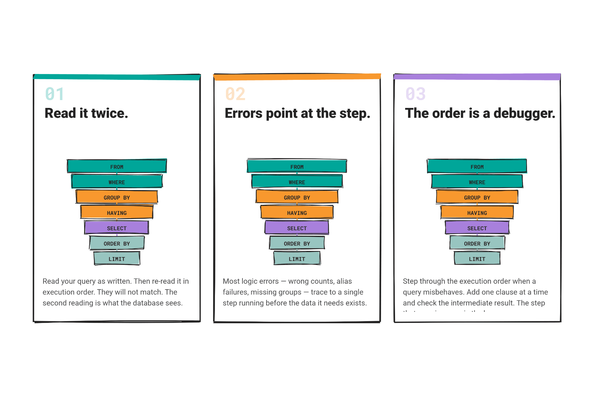
Three rules carry most of the value. Aggregate filters go in HAVING, not WHERE, because aggregates do not exist before grouping. SELECT aliases are only visible to ORDER BY, because everything else runs earlier. Window functions cannot sit in WHERE, so rank in a CTE and filter one level up. Each of the questions above shows one of these rules in a query you can run yourself.
When a query behaves in a way you did not expect, read it in execution order rather than top to bottom. The step where your mental model and the engine disagree is almost always where the bug is.
Frequently Asked Questions
Is SQL Execution Order the Same Across Databases?
The logical execution order of SQL is the same across PostgreSQL, MySQL, SQL Server, and Oracle because the SQL standard defines it. What differs is the final-step syntax (LIMIT versus TOP versus FETCH FIRST) and the physical plan the optimizer chooses at runtime. The conceptual order you reason with does not change.
Does SELECT Execute First or Last?
SELECT is written first but runs sixth, near the end. It runs after FROM, JOIN, WHERE, GROUP BY, and HAVING, and before DISTINCT, ORDER BY, and LIMIT. This is why output aliases are not available to earlier clauses.
When Should I Use WHERE vs HAVING?
Use WHERE to filter individual rows before grouping, and HAVING to filter groups after aggregation. If the condition tests a single row's column, it goes in WHERE. If it tests an aggregate like COUNT(*) or SUM(salary), it goes in HAVING.
Where Do Window Functions Fit in SQL Execution Order?
Window functions are evaluated around SELECT, after GROUP BY and HAVING, and before DISTINCT and ORDER BY. That placement is why you can order a window by an aggregate, and why you cannot reference a window function in WHERE.
Why Does WHERE Execute Before SELECT?
WHERE runs before SELECT so the engine can discard rows before computing output expressions over them. Filtering first reduces the rows that reach grouping and projection, and it means WHERE cannot depend on anything SELECT produces, including aliases.
Why Can't Aliases Be Used in WHERE?
An alias is created in SELECT at step 6, and WHERE runs at step 3. The alias does not exist yet when WHERE is evaluated, so you have to repeat the underlying expression in WHERE instead of using the alias name.
Why Does HAVING Work With Aggregate Functions?
HAVING runs at step 5, immediately after GROUP BY has computed the aggregates. Because the aggregate values already exist at that point, HAVING can compare against them. WHERE, running before grouping, cannot.
Does ORDER BY Execute Before LIMIT?
Yes. ORDER BY runs at step 8 and sorts the full result, then LIMIT runs at step 9 and keeps the first N rows of that sorted result. Without ORDER BY, LIMIT returns an arbitrary set of rows, because there is no defined order to slice.
Share