Statistics Cheat Sheet Part 03: Random Variables and Probability Distributions

Random Variables

In mathematical terms, a random variable is a number whose value is dependent upon the outcome of a random event. For example, if we define the random variable (X) to be the number of times, we get a head while tossing a coin twice.

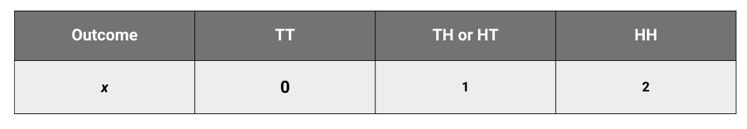
Note: We use uppercase to denote the variable and lowercase to denote a single value of X. Here, x = 1 when exactly one head comes up in two tosses of the coin.

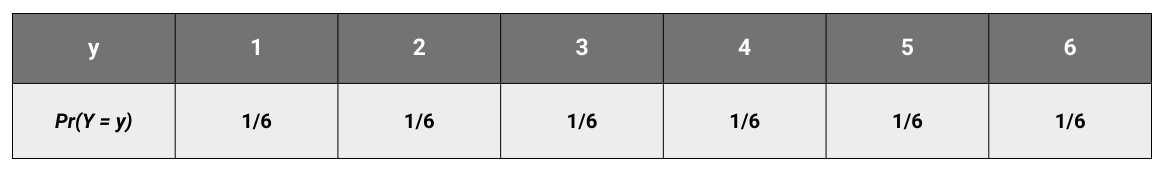
Let us take another example. Let Y denote the number that shows up in the roll of a dice. The random variable Y could be any number from 1 to 6.

Probability Distribution

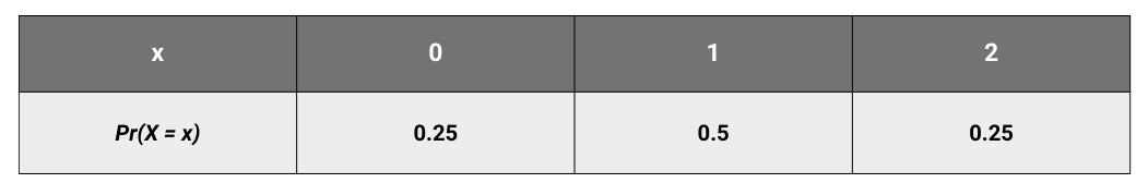
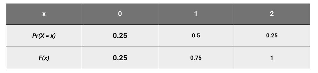
Let us write down the probabilities of the outcomes. The probability distribution for X (number of heads while flipping a coin twice) can be written as Pr(X = x). We get the following probabilities.

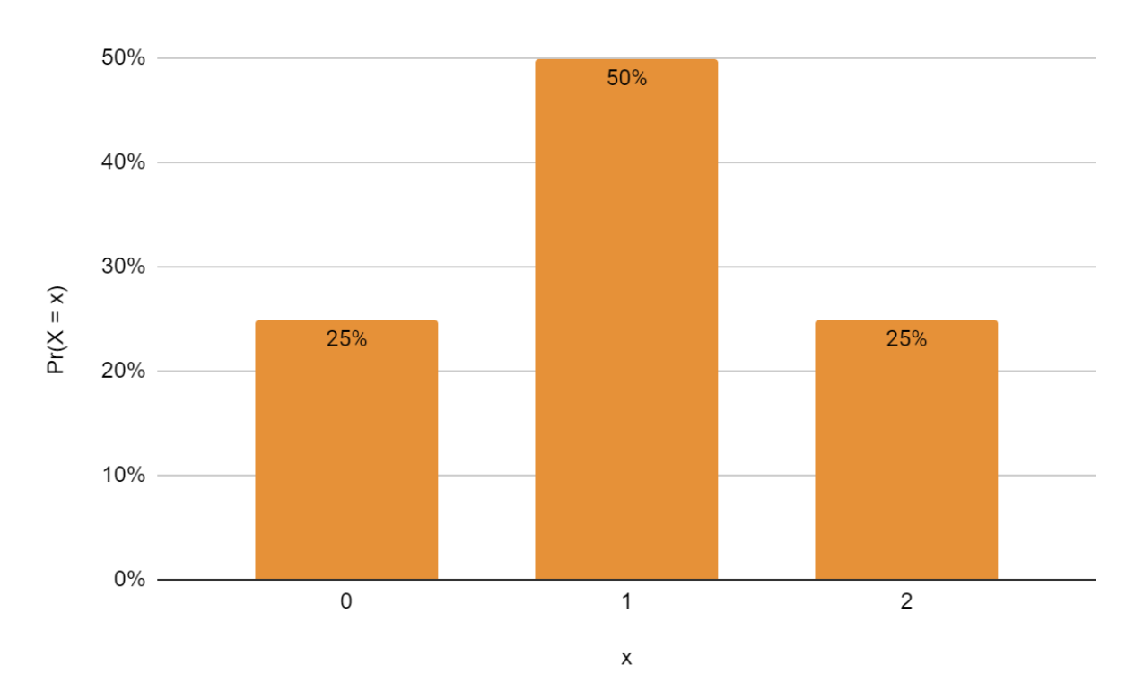
We can plot these values in a histogram

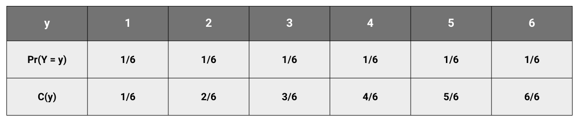
For the random variable Y (the number on the face of the die), the probabilities look like this.

And the histogram for Y looks thus.

The tables and histograms describe the probability distribution of the random variable.

A probability distribution is a mathematical description of the probabilities (or likelihood) of different outcomes in a random event.

Probability Mass Function

The examples we have considered till now have a finite number of outcomes. We cannot have 1.4 heads while tossing a coin twice. Therefore the probabilities associated with these outcomes, too, will be finite. The random variables are, therefore, Discrete Random Variables. The probability distribution for a discrete random variable is also called the probability mass function (PMF). We will look at continuous variables a little later in the article.

Cumulative Distribution Function

Another way of representing the probabilities associated with a random variable is to map the cumulative probabilities. A cumulative probability for a random variable X at value x is the probability that X takes a value less than or equal to x. Typically we use the uppercase F to represent a cumulative probability. Therefore F(x = a ) = Pr(X ≤ a). This function is called the cumulative distribution function (CDF). The advantage of a CDF is that it has the same definition irrespective of whether the variable is discrete or continuous. For the examples above, we can construct the CDF by just adding up the PDF.

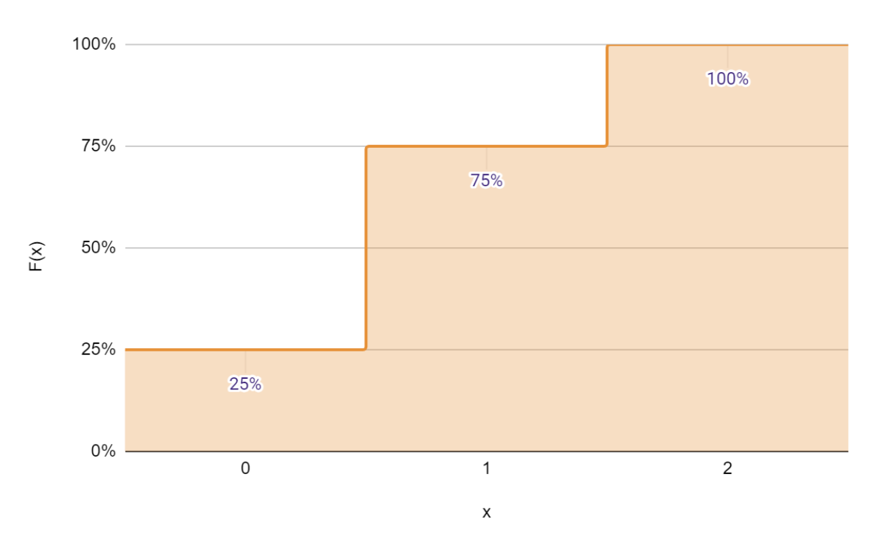
For our coin toss example

The CDF can be plotted thus.

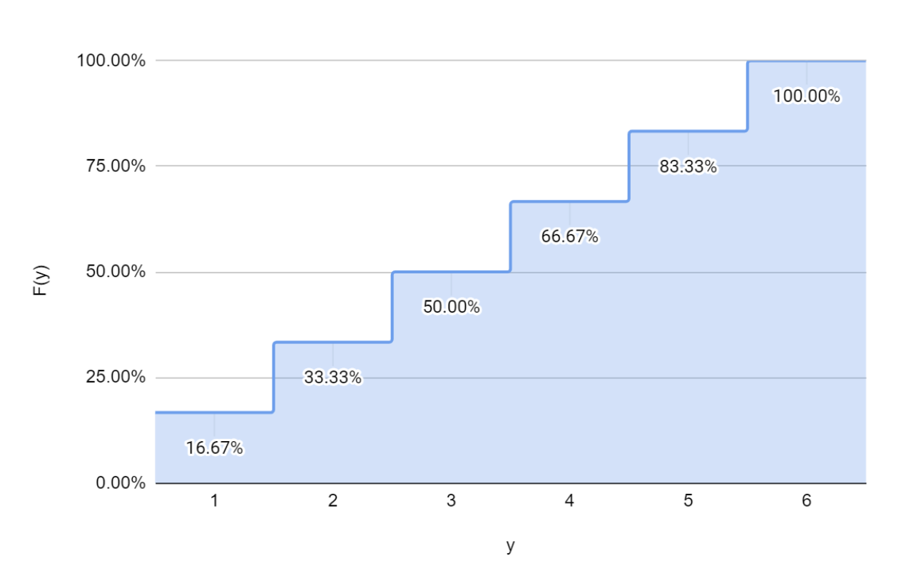
And for the die roll,

The CDF can be plotted as follows.

Discrete Probability Distributions

Theoretically, there can be infinitely many probability distributions. However, a handful of them appears so frequently that they merit special mention. Let us look at some prominent discrete probability distributions.

Uniform Distribution

The discrete uniform distribution describes a random variable that can take on a finite number of discrete values, with all values being equally likely. A very common example is tossing a coin once. Getting a head or getting a tail is equally likely. Another example is rolling a die. Each of the six numbers is equally likely.

Mathematically, the PMF of a Discrete Uniform Distribution is defined by two parameters, a, and b, where a is the minimum value the random variable can take and b, is the maximum. PMF is given by

P(x) = \frac{1}{b-a +1}

where x is the outcome of the random variable, and the values of x range from a to b, inclusive.

Applying this to the case of rolling a die

a = 1, b = 6

P(x) = \frac{1}{6-1 +1} = \frac{1}{6}

Binomial Distribution

The binomial distribution describes the number of successes (x) in a fixed number of trials or repetitions (n). Each of the trials has only two possible outcomes: success or failure. Further, the probability of success in a given trial always remains constant. Let us call it p. Each of these trials or repetitions is called a Bernoulli trial. The probability distribution is given by

Pr(X = x) = {n \choose x}p^x (1-p)^{n-x}

where x is the number of successes in n trials,

{n \choose x}

The above denotes the binomial coefficient given by

{n \choose x} = \frac{n!}{x! (n-x)!}

Application of the Binomial Distribution

In an office, 80% of the employees arrive between 8 AM and 9 AM. Find the probability that on a given day, at least seven of the ten employees will arrive between 8 AM and 9 AM.

There above problem represents a Binomial Distribution with 10 trials and a probability of success of 80% or 0.8.

We need to calculate the probability that X ≥ 7. Therefore, we need to calculate

P(X = 7) + P(X = 8) + P(X = 9) + P(X = 10)

Applying the binomial formula, we get

P(X = 7) = \frac{10!}{7! (10-3)!} (0.8)^7 (1-0.8)^{10-7} = 0.201

Similarly

P(X = 8) = 0.302
P(X = 9) = 0.268
P(X = 10) = 0.107

Therefore P(X ≥ 7) = 0.201 + 0.302 + 0.268 + 0.107 = 0.878 or 87.8%

Geometric Distribution

The Geometric Distribution builds on the Binomial Distribution. Here the trials (or repetitions) continue until success occurs rather than a set number of trials. Theoretically, the trials can continue indefinitely. For example, suppose you keep rolling a die till you get the number 6. In theory, we might go on an extremely unlucky streak and not get a six.

The PDF for a geometric distribution is given by

P(X = x) = p (1-p)^{x-1}

Where X denotes the number of repetitions needed to get the first success.

This is the PDF of a Geometric Distribution with p = 0.2.

Application of the Geometric Distribution

In a town, 60% of the population is female. Find the probability that a person will need to meet three people before meeting the first male.

Let us write the problem down in simple English.

The probability that only the third person we will meet is a male is

Probability that the first person we meet will be a female and the second person we meet will be a female, and the third person we meet will be a male

Now it is easier to calculate the values. The probability of meeting a female is 60%, and the probability of meeting a male is (100 - 60)% = 40%

Therefore, the required probability = 60 % x 60 % x 40% = 14.44%

Alternatively, we could use the formula. Here x = 3 and p = 40% or 0.4

Therefore

P(X = 3) = 0.4 . (1-0.6)^2 = 0.144

or 14.44%

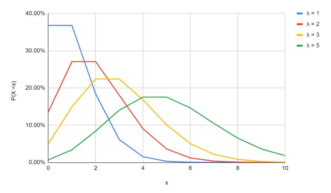
Poisson Distribution

Another very common discrete distribution is the waiting time distribution or the Poisson Distribution. Poisson distribution describes the probability of a given number of events occurring in a fixed interval of time or space if these events occur with a known average rate and independently of the time since the last event. The common applications include finding how many lines a shopping center should keep so as not to overload the system. There is only one parameter needed - the average number of occurrences during the interval period. This parameter is usually represented by λ.

The Probability Distribution for a Poisson Process is given by

P(x) = \frac{(\lambda^x e^-\lambda)}{x!}

where λ is the average number of occurrences in the interval, x is the number of occurrences of the event (or successes) in the given interval, e is the natural logarithm (approximately 2.718).

The PDF of a Poisson Distribution with different values of λ

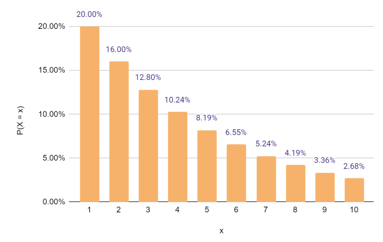
Application of the Poisson Distribution

It is observed that a WhatsApp group gets 45 messages per day. What is the probability that it will receive more than two messages in the next half hour?

Our time frame (or interval) of interest is half an hour. We start by calculating the average number of messages received every half hour.

In a day, there are 24 hours, so 24x2 = 48 half-hour periods.

The average number of messages received each half hour (λ) =

\frac{45}{48} = 0.9375

We need to find P(x > 2). We can find this by

P(x > 2) = 1 - P(x\le 2) = 1 -[P(x=0) + P(x=1) + P(x=2)]

Plugging in x = 0, 1, 2 and λ = 0.9375 into the formula, we get

P(x > 2) = 1 - {[\frac{(0.9375^0e^{-0.9375})}{0!} + {[\frac{(0.9375^1 e^{-0.9375})}{1!}} + {[\frac{(0.9375^2 e^{-0.9375})}{2!}} ]}

P(x > 2) = 1 -[0.3916+0.3671+0.1721] = 1-0.9308 = 0.0692 = 6.92\%

Continuous Probability Distribution

Till now, we have looked at variables that have a finite set of values (Heads or Tails on a coin, Number on the face of a die, etc.) only. But in real life, variables can have infinitely many values. Let us take the case of a person arriving between 1 PM and 2 PM for a lunch appointment. Assuming that a person can come any time, the chances of him arriving between 1:10 and 1:30 PM can be calculated as

Favorable time period = 1:10 PM to 1:30 PM = 20 minutes

Total time period = 1 hour = 60 mins.

Therefore probability = ⅓..

However, if you want to calculate the probability of him arriving exactly at 1:15 PM, it will depend on how accurately we measure time. If we are measuring by rounding to the nearest minute, it will be 1 in 60. If we measure to the last second, then it will be 1 in 3600. If we measure in milliseconds, then 1 in 3.6 million and so forth. As you can see, the exact moment of arrival can be split into further smaller segments. It can take infinitely many values. Therefore the probability of him arriving at a given point in time is zero.

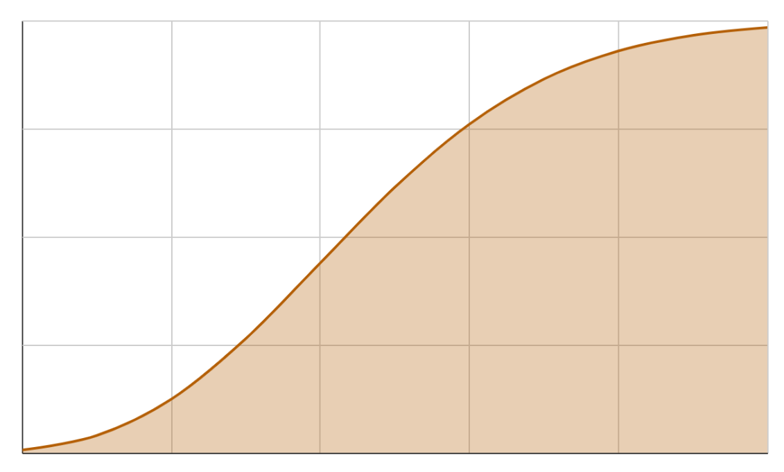
Such variables are called continuous variables. Formally if you draw the cumulative distribution function (CDF) for a continuous random variable, it will not have any breaks (or steps) that we saw earlier in, say, rolling a die.

The CDF for a continuous variable will look like this.

For continuous random variables, we find the probability for intervals (as in the case of arrival times described above) rather than individual values. While the math is a bit tricky as it involves calculus, intuitively, we can use the concepts from discrete random variables for continuous variables as well since we can convert a continuous random variable to a discrete one by rounding off (as we did in the seconds to the minute example described above).

Probability Density Function

As we have seen, the probability of a continuous random variable at a particular value is always zero. Therefore for continuous variables, we find the amount of change in CDF at any instance. This change is called the Probability Density Function. In terms of calculus, PDF is the differential of CDF. The PDF of the continuous random variable will look like this.

To find the probability between two points, we find the area under the curve (integrate the PDF over these two points using integral calculus). Luckily, we do not need to do that. We can easily calculate these values using Python or any spreadsheet software.

Note: For any continuous probability distribution,

P(a ≤ x ≤ b)\ ≣\ P (a < x < b)\ ≣\ P(a ≤ x < b)\ ≣\ P(a < x ≤ b)

This is because the exact probability at a particular value is always zero.

Continuous Uniform Distribution

As with discrete uniform distribution, for a continuous uniform distribution too, the events are equally likely to occur. Only the range of values possible is infinitely many.

The PDF for continuous distribution is given by

P(x) = \frac{1}{b-a}

for a ≤ x ≤ b

where a is the lowest possible value, and b is the highest possible value.

Application of the Continuous Uniform Distribution

It takes between five to fifteen minutes for a cab to arrive after it is booked on the Suber app. What is the probability that a customer will have to wait for more than twelve minutes for a cab?

Let us try this to solve this without using a formula. Similar to the PMF for discrete uniform distribution, we can draw the PDF for the continuous one.

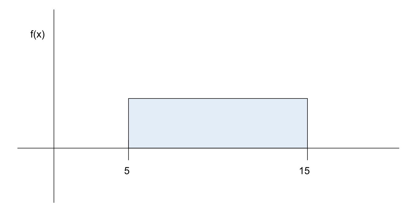
The area under the whole curve should be equal to 1 since it is certain that the cab will come within this time period. The width of the rectangle is 15 - 5 = 10 units. Since the area is 1, the height should be below which is = 0.1.

\frac{1}{10}

To find P(x > 12), we can find the area of the shaded portion P(5 ≤ x ≤ 12) and subtract from 1.

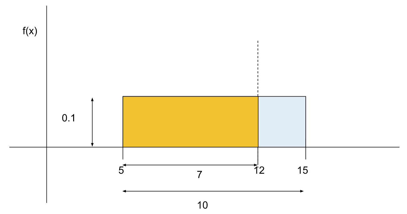
Area of the shaded portion

=\ 7\ x\ 0.1 = 0.7 = P(5 ≤ x ≤ 12)

Therefore,

P(x > 12) = 1 - P(5 ≤ x ≤ 12) = 1 - 0.7 = 0.3 = 30\%

Exponential Distribution

Another continuous distribution commonly encountered is the exponential distribution. It models the amount of time until a specific event has occurred. For example, the time taken to service a customer, how long a part would last before it has to be replaced, etc. The PDF for an exponential distribution is given by

f(x) = me^{-mx}

where m is called the decay factor. It is calculated as the reciprocal of the historical average waiting time.

The CDF for the distribution is given by

F(x) = 1- e^{-mx}

Application of the Exponential Distribution

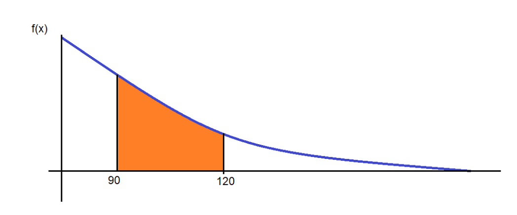
On average, a car has to be serviced after 120 days if used every day. The time for servicing can be modeled using an exponential distribution.

What is the probability that the car will be serviced after 150 days?
What fraction of cars will be serviced after 90 days but less than 120 days?

Here the decay factor (m) =

\frac{1}{120}

Let us solve part A first.

We need to find P(x > 150). The required probability is given by the shaded area in the portion.

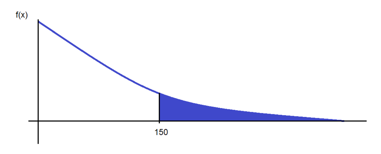
In this case, it is easier to find the area of the unshaded area. If you recollect the discussion on CDF, the area of unshaded area is CDF (X = 150). Once we find that, we can simply subtract that from 1 to find the area of the shaded portion.

Since we already have the CDF function, we can rewrite the required probability as

P(X > x) = 1 - CDF (X = x) = 1 - (1 - e^{-mx}) = e^{-mx}

In this case, x = 150. And the decay factor

m = \frac{1}{120}

Plugging the values, we get

P(X > 150) = 0.2865 = 28.65\%

This feels intuitively right - since most cars have to be serviced after 120 days, very few cars will have to be serviced after 150 days.

With this done, we can also solve Part B similarly.

Part B asks us to find the probability that a car will be serviced between 90 and 120 days or P(90<X<120). Graphically, the area of the shaded portion is the required probability.

We can break this down as

P (X < 120) - P(X ≤ 90)

Again, we will use the property of CDF to find these values.

P (X < 120) = CDF(X = 120)\ and\ P (X ≤ 90) = CDF (X = 90)

Therefore

P(90<X<120) = CDF(X = 120) - CDF (X = 90)

Graphically this can be represented in the following manner.

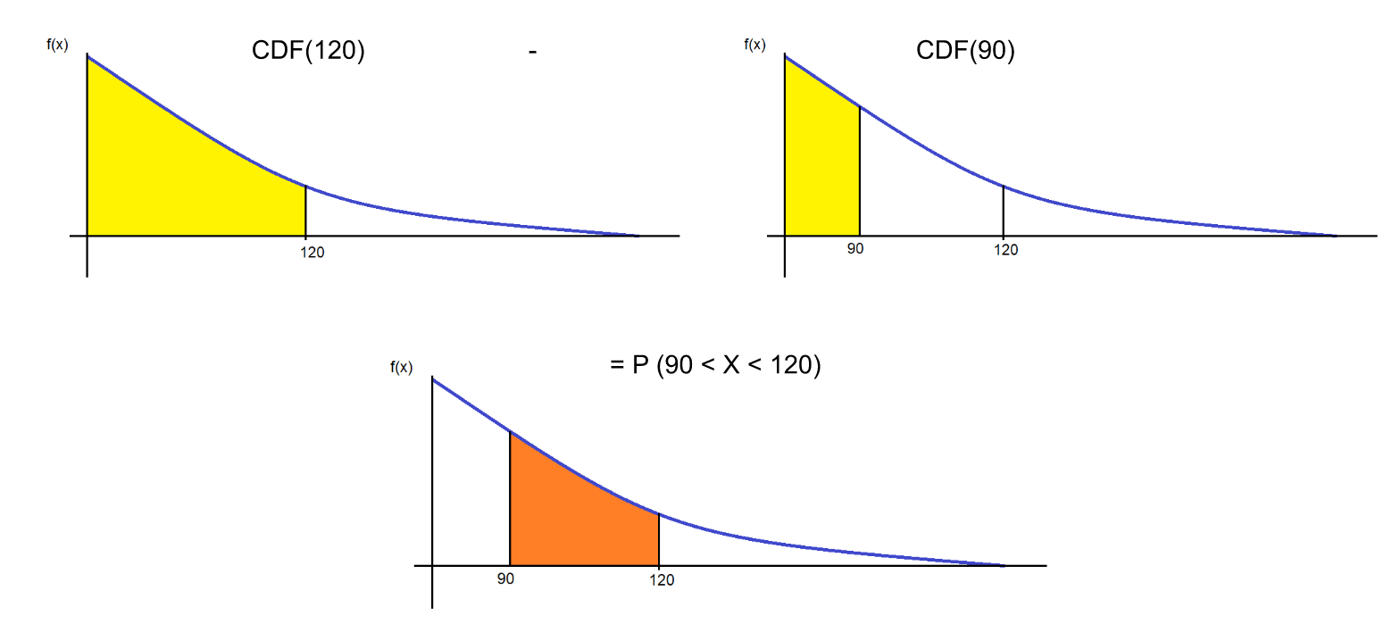
We can now calculate the probabilities easily.

CDF(X = 120) = 0.6321
CDF(X = 90) = 0.5276
P(90 < X < 120) = 0.6321 - 0.5276 = 0.1045 or 10.45%

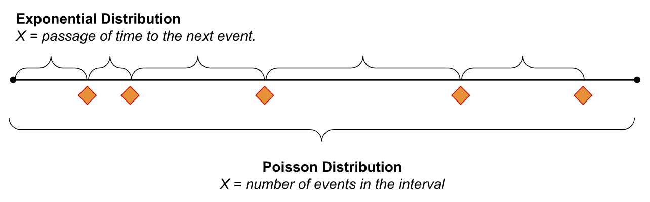
Comparison of Poisson Distribution and Exponential Distribution

The decay factor m in Exponential Distribution is the inverse of the average occurrence time λ of the Poisson Distribution. However, there are some differences. In the Poisson Distribution, the random variable x (number of occurrences in the given time period) is discrete. However, in the exponential distribution, the random variable x (the time for the next success) is continuous.

To relate this to an example from the WhatsApp group we did earlier. The number of messages that we receive in a particular time period is a discrete variable and can take positive integral values only (0, 1, 2, 3, … ); while the time to the next message is a continuous variable and can take fractional values as well (2.3 minutes, 4.8 hours, etc.). The difference can be illustrated in the figure below.

Comparison of Poisson Distribution and Exponential Distribution

Normal Distribution

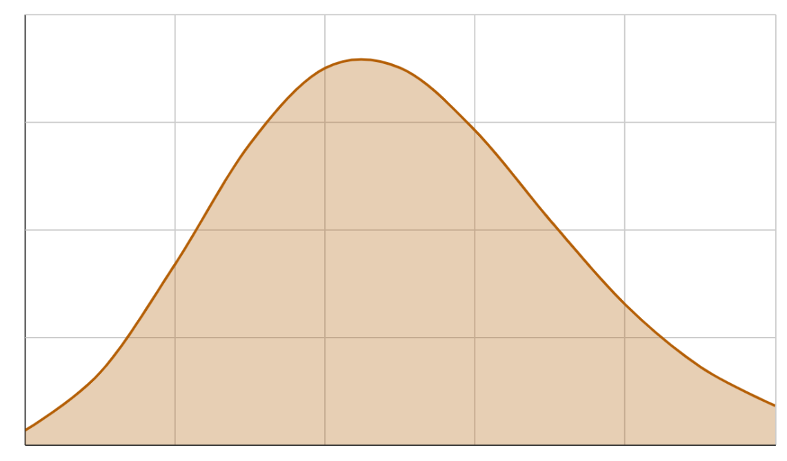
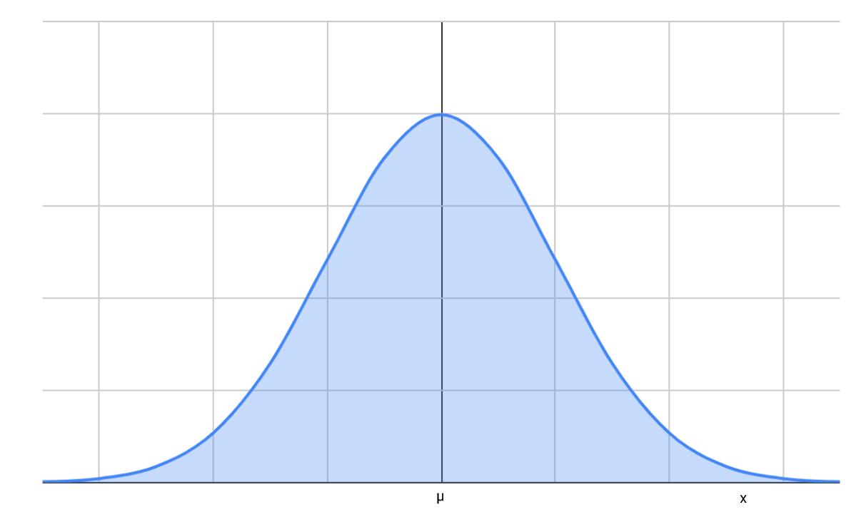
Irrespective of your academic or professional background, you would have heard of Normal Distribution. It is one of the most used (and abused) probability distributions. Understanding Normal Distribution is critical to the understanding of inferential statistics. The normal distribution has a bell-shaped curve described by the following PDF

f(x) = \frac{1}{\sigma\sqrt{2\pi}} e^{-\frac{1}{2}\left(\frac{x-\mu}{\sigma}\right)^{\!2}}

Here μ is the mean of the distribution and σ the standard deviation.

The graph of the PDF of Normal Distribution looks like this. The graph is symmetrical around the mean.

Note: You do not need to memorize the formula. Just how to use it.

Since the area under the curve must be equal to one, a change in standard deviation results in the fatter or taller curve depending on σ

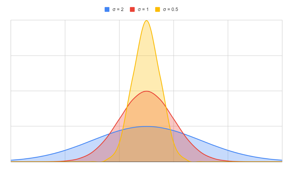
We can therefore have infinitely many Normal Distributions.

Standard Normal Distribution

A Standard Normal Distribution has a mean of 0 and a standard deviation of 1. We can convert any normal distribution with mean μ and standard deviation σ to the standard normal distribution by performing a simple transformation.

z = \frac{x - \mu}{\sigma}

The z-score tells how many standard deviations is x away from the mean.

This ensures that we just need one table like this to take care of all our probability calculations. This was before the advent of spreadsheets and statistical programs, but it is still very helpful.

How to use z-scores to find probabilities?

Most software will be able to provide us with PDF and CDF values very easily. For the sake of better understanding, let us use the z-score table as provided here.

As the heading suggests, the table provides us with the area to the left of the z-score.

How to use z-scores to find probabilities

In other words, the table gives us CDF values at a particular z-score. Therefore, if we want to find the probability of P(z < -1.63), we can directly read this directly off the table as described in the figure below. First, we read the first two significant digits (-1.6) vertically and then read the last digit (3) horizontally. Therefore CDF (z = -1.63) = P (z < -1.63) = 0.05155 or 5.155%.

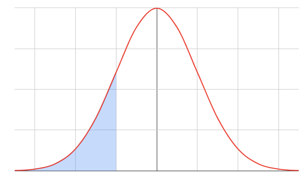
If we want to find out P (-1.8 < z < 1.2), we can do it in the same manner as we did for the Exponential distribution earlier.

P (-1.8 < z < 1.2) = CDF ( z < 1.2) - CDF ( z ≤ -1.8)

Reading the values off the table,

P (-1.8 < z < 1.2) = 0.88493 - 0.03593 = 0.849 or 84.9%

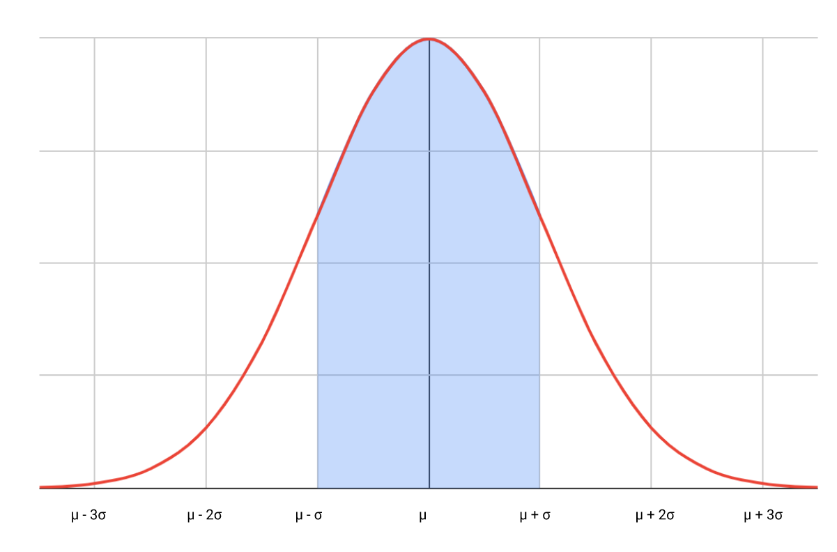
The Empirical Rule of Normal Distribution

For any normal distribution with mean μ and standard deviation σ, the empirical rule states that

The area within one σ either side of the mean is approximately 0.68. In other words, 68% of the time, you can expect x to be within μ - σ and μ + σ

We can find this very easily using the z-score tables. We start off by transforming the x values to z-scores. A value of x = μ + σ will give us a z-score of

z = \frac{\mu + \sigma - \mu}{\sigma} = 1

Similarly, a value of x = μ - σ will translate to a z-score of -1

We can now find the area between these two z-scores by using the CDF tables as earlier

The Empirical Rule of Normal Distribution

P (-1 < z < 1) = CDF ( z < 1) - CDF ( z < -1) = 0.84134 - 0.15866 = 0.68269 or 68.27%

Similarly, around 95% of the time, x to be within μ - 2σ and μ + 2σ
And, around 99.7% of the time, x to be within μ - 3σ and μ + 3σ

Let us use Normal Distribution in real life.

Application of Normal Distribution

If it is known that the average weight of adult men in Europe is 183 pounds with a standard deviation of 19 pounds. What fraction of adult men in Europe weigh more than 160 pounds but less than 200 pounds?

Given: μ = 183, σ = 19. We need to find P (160 < x < 200).

This problem can be solved as earlier by finding converting the x values to z-scores.

For\ x\ = 160,\ z = \frac{160-183}{19} = -0.684

For\ x\ = 200,\ z = \frac{200-183}{19} = 0.895

The problem, therefore, reduces to

P (160 < x < 200) = P (-0.684 < z < 0.895)
= CDF (0.895) - CDF(-0.684)
= 0.8146 - 0.2470
= 0.5676 or 56.76%

Conclusion

In this article, we looked at the basic terms and techniques involved in working with random variables. We also looked at the different probability distributions for discrete and continuous random variables and finished off by working with normal distribution. In the next article, we will extend these concepts to the field of inferential statistics. We have many problems on probability theory and statistics on the StrataScratch platform. Join a community of more than 20,000 aspirants aiming to get into the most sought-after Data Science roles at companies like top companies like Apple, Meta, Amazon, Netflix, etc.