Statistics Cheat Sheet Part 02: Probability and Random Events

A beginner’s guide to Probability and Random Events. Understand the key statistics concepts and areas to focus on to ace your next data science interview.

In our previous article on statistics, we looked at the different pillars of statistics. We went through the various data collection methods to understand the population characteristics. We also explored the world of descriptive statistics. We went through various measures of central tendency and measures of spread. In this session, we will look at concepts from probability and random events. Also, check out our comprehensive “Statistics Cheat Sheet” for important terms and equations for statistics and probability. You can also look at our top probability interview questions to find out the nature of questions asked in Data Science Interviews.

Probability

Probability is a branch of mathematics estimating how likely something is going to happen. Probability theory is applied in everyday life in risk assessment and modeling. For example, the premiums for car insurance are determined by how likely an adverse event like an accident or breakdown is likely to happen. If you have a poor driving record or a very old and poorly maintained vehicle, you will have to pay a higher premium compared to a person with a faultless driving history and a new car. Probability is the backbone of all Data Science Models and it is critical that one understands probability theory.

Random Events

A random event is something that will happen. For example, your car might be involved in an accident. It matters to you since it is your car. It also matters to your car insurer since they have to bear the costs if an accident happens. However, we do not know in advance that it will happen. The outcome of the event can be a simple True / False result example - Did Biden win the presidency? Or it can be more complex like was the driver wearing a seat belt, not driving under influence, and within speed limits when the accident happened? Whatever the outcome, it should be complete in the sense that everything that we are interested in can be defined in terms of the outcome.

Basic Definitions

Elementary Outcomes are all the possible results of a Random Event. For example, while tossing a coin, getting a head would be an elementary outcome. So is getting a tail. In the case of rolling a six-faced dice, each of the numbers would represent an elementary outcome.

Sample Space (Also called Possibility Space) is the set of all elementary outcomes. For example, tossing a coin once, the sample space is {H, T}. If we were tossing two coins, then the sample space would be {HH, HT, TH, TT}.

Probability

P(H) = P(T) = 0.5

Probability can be defined as

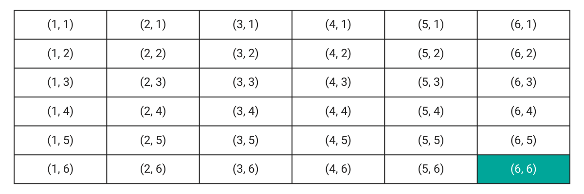
In the case of rolling two six-faced dice simultaneously, the sample space can be viewed in the following manner.

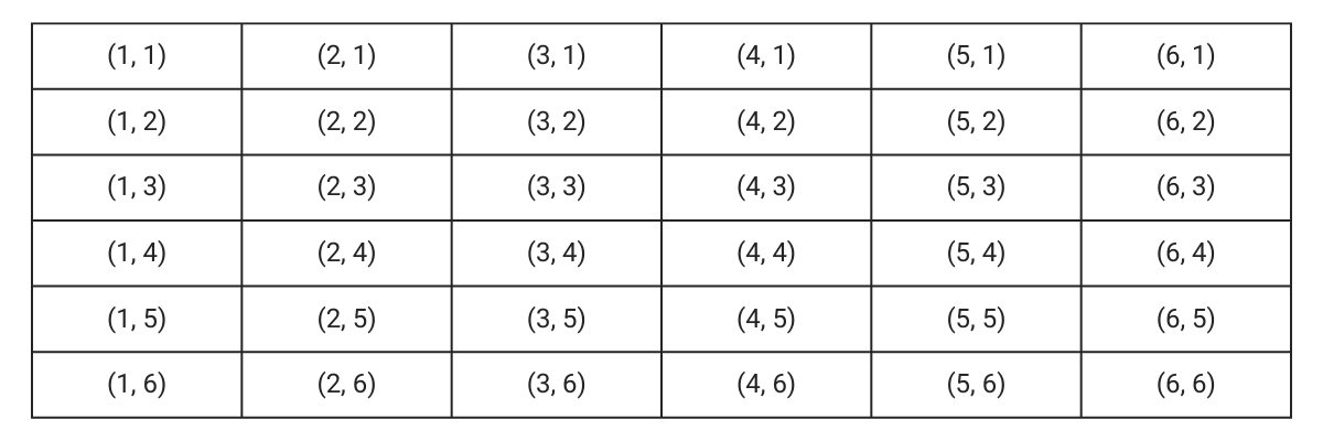
Each of the above outcomes is equally likely. Therefore the probability for each is:

What this means is that if you keep rolling two dice a very large number of times, each of these outcomes would occur the following of the time:

Note: in the above case, we consider (3,6) and (6,3) as two different outcomes. In the former, the first dice shows a 3 and the second a 6. In the latter, the numbers are reversed.

Characteristics of Probability

Probability is non-negative. Think of probability as the battery level on your phone. If the level is low, there is a lesser chance that the outcome will occur, if the level is high, the greater the chances. As with your phone battery, it cannot go below zero.

The probability of an outcome always lies between 0 and 1 (both inclusive).

• If the probability of an outcome is 0, then it is an impossible outcome.
• If the probability of an outcome is 1, then it will definitely happen.

Further, the sum of all probabilities of all possible outcomes equals 1. In other words, one of these outcomes will definitely happen.

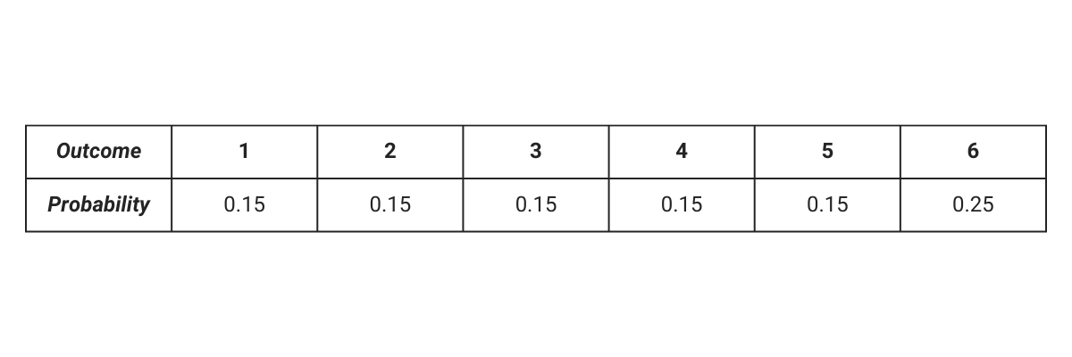
Note: The elementary outcomes need not have equal probabilities. For example, suppose we load a die to make sure that the number 6 comes 25% the following of the time:

Instead of as earlier:

The sample space remains the same, {1,2,3,4,5,6}.

All the probabilities add up to 1, we get the following

P(1) + P(2) + … P(5) + P(6) = 1

We know that P(6) = 0.25 and all the other outcomes have equal probabilities: P(1) = P(2) = .. P(5). We can therefore rewrite the above as

We get the following probabilities for each of the outcomes of the loaded die. As you can verify the sum of the probabilities add up to 1.

Operations

Till now we have discussed the probability of elementary outcomes. However, in practice, these can become pretty unwieldy. If we were to find the probability of getting a sum of 6 by adding up the numbers on the dice. This is not an outcome in the sample space. To find the probabilities, we extend the elementary outcomes to events. In probability theory, an event is a group of outcomes. A subset of the sample space. So let us add up the numbers on the faces of two dice for all cases.

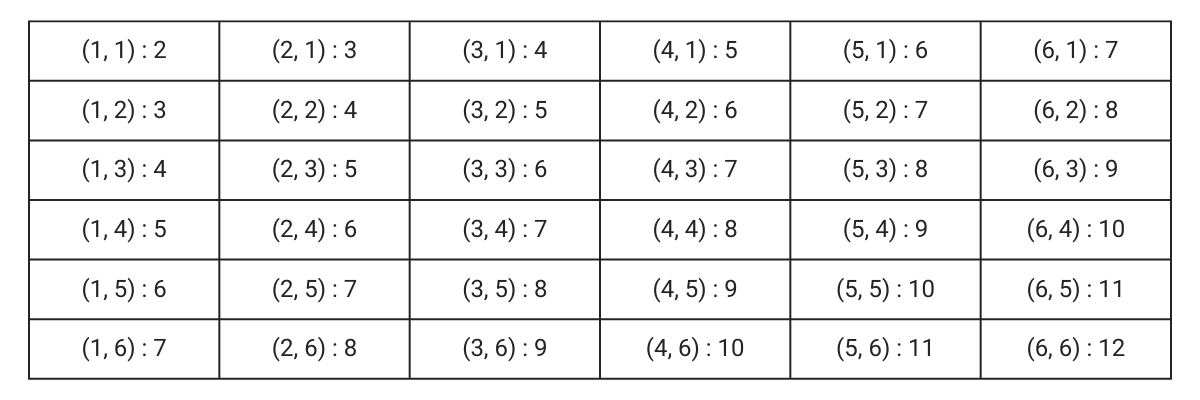
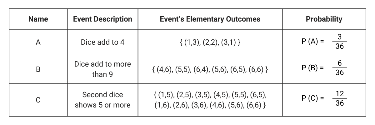
To find the probability of events, we simply add up the probabilities of the elementary outcomes that satisfy the conditions of the event. Here are some of the events and their associated probability.

The advantage of using events rather than elementary outcomes is that we can combine events using logical operations AND, OR and NOT to form more events. So for any two events X and Y, we can make new events in the following manner.

X AND Y: Both event X and event Y occur
X OR Y: At least one of event X or event Y occurs
NOT X: Event X does not occur

Combining the definitions of probability with these logical operations gives us more powerful formulae for manipulating probabilities. Let us look at the two-dice situation.

Event X: The first die shows 3
Event Y: The second die shows 3.

The blue box shows event X, while the red box shows event Y. The overlap event X AND Y (3 shows up on both the dice) is the overlap.

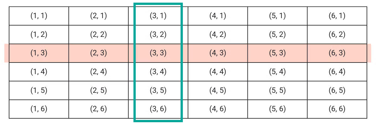
If we have to find out the probability that one of the two dice shows 3 : P(X OR Y), we cannot simply add P(X) and P(Y) because we will be double counting the elementary outcomes shared by X and Y. This gives us the addition rule for probability.

P (X OR Y) = P(X) + P(Y) - P(X AND Y)

We can verify the addition rule for the above example.

There are times when there is no overlap. For instance, suppose we want to find the probability of getting a total of 3 (orange) or a total of 9 (green).

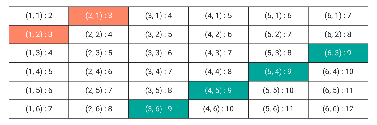
These events are mutually exclusive events and P(X AND Y) is 0. In such cases, we can modify the addition rule to

P(X OR Y) = P(X) + P(Y)
X, Y are mutually exclusive events

We can verify this.

Sometimes it is easier to calculate when an event has not happened. For example if we want to find out the probability that none of the dice show a 3.

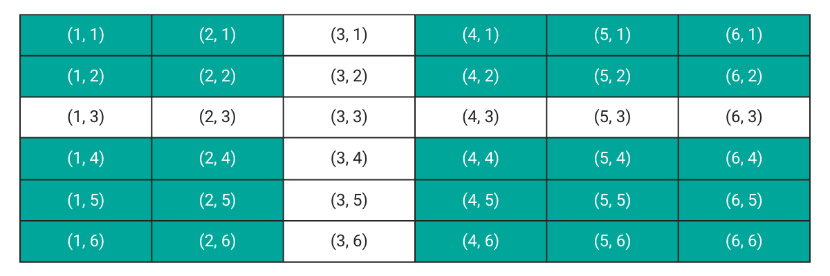
The shaded area contains the favorable cases. This is the complement of the earlier problem where we calculated the probability that at least one of the dice shows a three. We can simply use the complement rule which states that

P (NOT A) = 1 - P(A)

We have already calculated the probability that at least one of the dice shows a 3

Therefore the probability that none of the dice show a 3 would be

Conditional Probability

Let us alter the process a little bit. Instead of throwing both the dice together, we throw the dice one after the other, noting the number on the first die before we throw the second die. Before the dice are thrown, the probability of getting a sum of 9 (let us call this event A) will be

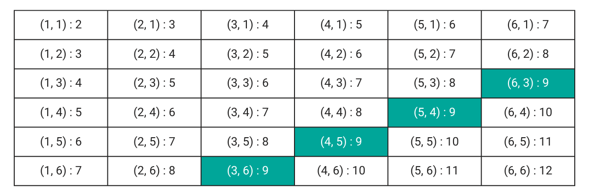
Suppose the first die shows a 6 (Let us call this event B). What is P (A) now?

We call it the conditional probability that Event A will occur, given that Event B has already occurred. We denote this P (A | B) : The probability of A, given B.

Since B has already occurred, the outcome is now only the number on the second die. The reduced sample space is now

Only one outcome (6,3) sums up to 9. So the conditional probability P (A | B) is

The formal definition of conditional probability of A, given B is

Resolving this, we get the Multiplication Rule.

P (A AND B) = P(A | B) P (B)

Independent Events

If the occurrence of one event has no influence on the occurrence of another, the two events are said to be independent events. For instance, while rolling two dice together, the outcome of the first dice has no influence on the outcome of the second roll, unless they are attached. In terms of conditional probability this is the same as

P (A) = P (A | B)

This is the same as saying that the probability of A does not change given B has occurred. And equivalently, P(B) = P(B | A)

When two events are independent, we get the multiplication rule

P (A AND B) = P (A) P (B)

We can use this to find the probability of getting a double 6 as the outcome while rolling two dice.

If we take

Event A: Number on the first die
Event B: Number on the second die

We can verify this from the table.

In our earlier example where we wanted to find the probability that the sum of dice add up to 9, obviously, the first die showing 6 affects the chances. We can verify this.

Event A: Sum of the dice is 9Event B: 6 shows up on the first die

Since P (A | B) ≠ P (A) the two events are not independent.

Let us see how conditional probabilities can be used to make real-life meaningful decisions.

A Better Speed Gun

From past data, around 5% of the vehicles drive above the speed limit. The traffic police are testing a new speed gun. The new speed gun can correctly identify 90% of all speeding cases. In other words, if a vehicle is speeding it will be detected 90% of the time. However, this speed gun also incorrectly identifies 20% of non-speeding cases as speeding cases. What is the probability that a vehicle stopped for a speeding violation using this speed gun was actually speeding?

We have two events to work with

A: The vehicle is speeding
B: The speed gun says that the vehicle is speeding.

For the data about the effectiveness of the speed gun, we can write down the following cases.

P (A) = 5% (Only 5% of the vehicles speed)
P (B | A) = 90% (The speed gun can detect 90% of the speeding cases)
P (B | NOT A) = 20% (The speed gun falsely tags 20% of non-speeding cases as speeding cases)

We need to find
P (A | B)  The probability that the vehicle was actually speeding given that the speed gun tags the vehicle as speeding.

We start by dividing the sample space into four mutually exclusive events.

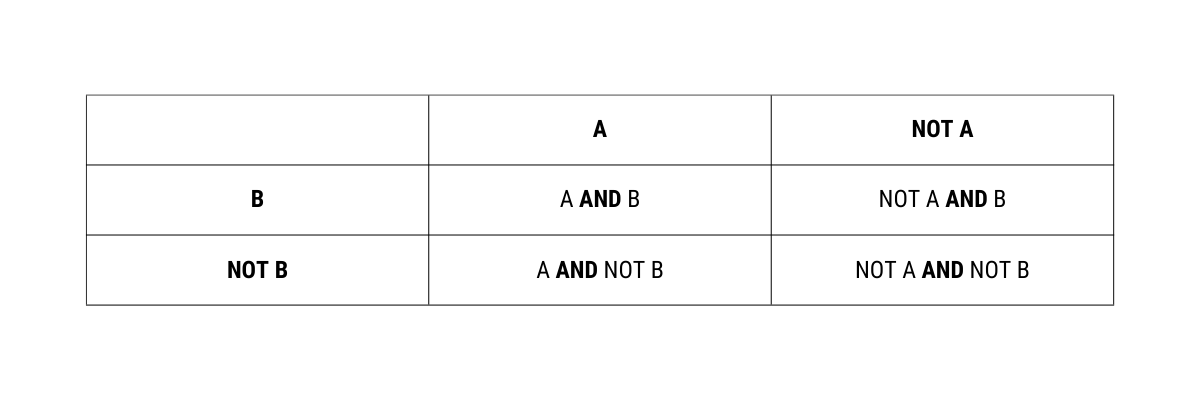
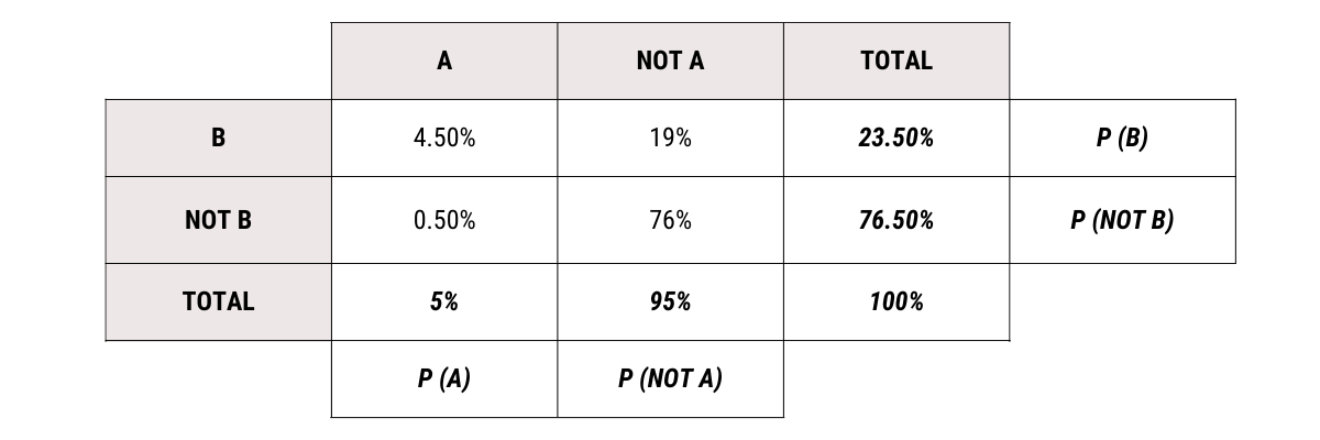
The table is called a contingency table (or cross-tabulation) and is very helpful in calculating probabilities. Let us find the probabilities in each case

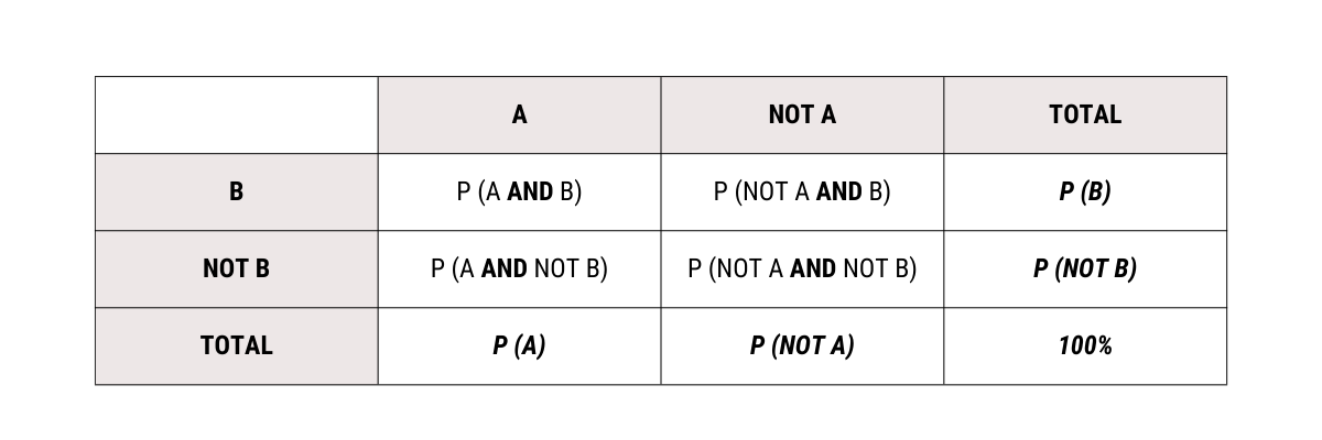
The totals are found by summing across rows and down the columns. Let us use the multiplication rule for conditional probabilities.

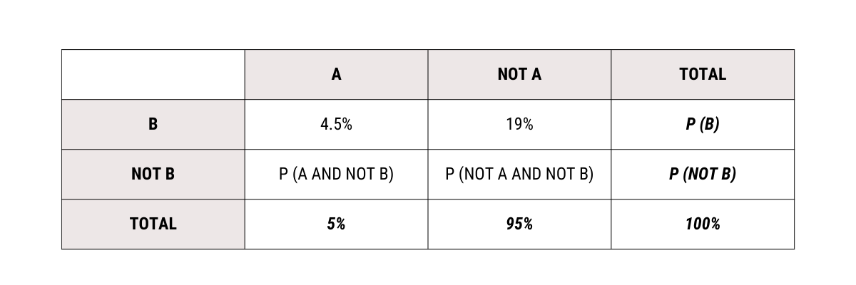
P (A AND B) = P (B | A) P (A) = (90%) (5%) = 4.5%
P (NOT A AND B) = P (B | NOT A) P (NOT A) = 20% * (100 - 5)% = 19%

Filling these into the contingency table.

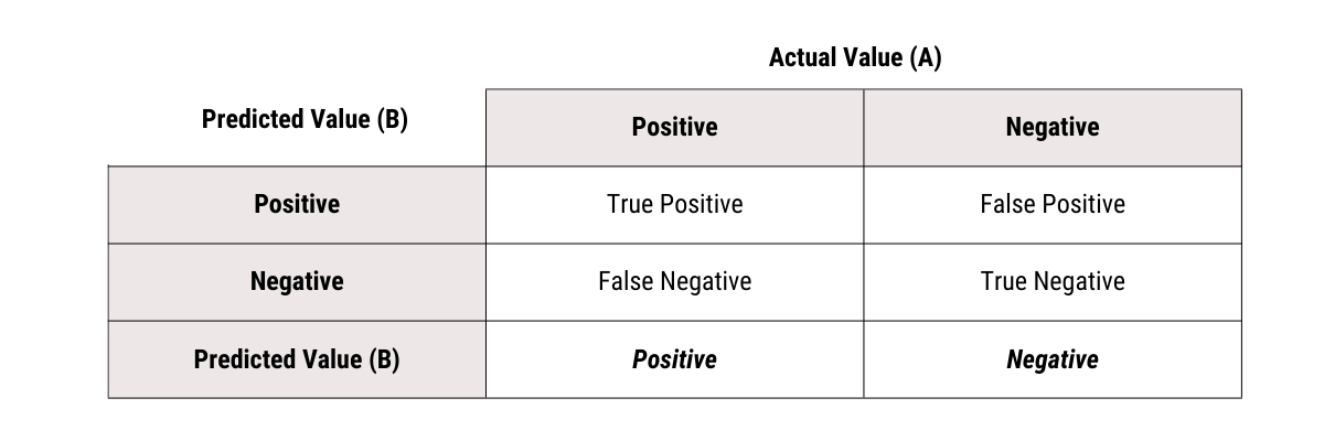
A cross-tabulation like the above is used to test the effectiveness of classification models. Replacing A with actual values and B with the prediction made by the speed gun, we get what is called a confusion matrix (or error matrix)

Let us come back to our problem. We can now find the remaining values.

P ( A AND B) = P (A | B) P (B)

4.5% = P (A | B) * 23.5%

Despite the high accuracy of the speed gun, less than 20% of those detected for speeding actually speed. This is called the False-Positive Paradox. Broadly, this describes a case where the false positives are more than the true positives because these characteristics are relatively rare in the general population. This is one of the reasons why doctors always rely on multiple tests to detect rare diseases.

Bayes’ Theorem

All the steps used for computation above can be compressed into a single formula called the Bayes Theorem.

This can be simplified by using the multiplication rule.

P (A) P (B | A) = P (A AND B)
P (NOT A) P (B | NOT A) = P (NOT A AND B)

We can also write

P (A AND B) + P (NOT A AND B) = P (B)

Thus Bayes’ Theorem can also be written as

As we saw above, Bayes' Theorem and conditional probabilities are very helpful in finding the probability of an event based on prior knowledge of conditions that might be related to the event. A prime example is in the field of health care where increasing age can lead to complications. Rather than assessing everyone identically, a more accurate assessment can be arrived at by taking the age into account.

Conclusion

In this article we looked at the basics of probability and random events. We used these concepts to move from outcomes to events and then explored the various characteristics of probability. We then used the concept of conditional probability to find independent events and finally used it in a real-life scenario. In the next article, we will expand this understanding to random variables and probability distributions.

Probability is fundamental to Machine Learning and Data Science and every aspiring Data Scientist should have a solid understanding. While it might look a bit difficult in the beginning because we are used to certainties in life, it is very intuitive. With a little bit of practice and persistence, one can easily become proficient in understanding various concepts. You apply your Probability and Statistics skills trying to solve data science interview questions on the StrataScratch platform. Join StrataScratch today and make your dream of joining companies like Netflix, Apple, Microsoft, Amazon, et al a reality.