A Comprehensive Statistics Cheat Sheet for Data Science Interviews

About This Statistics Cheat Sheet

When I was applying to Data Science jobs, I noticed that there was a need for a comprehensive statistics and probability cheat sheet that goes beyond the very fundamentals of statistics (like mean/median/mode).

And so, I'm going to cover the most important topics that commonly show up in data science interviews. These topics focus more on statistical methods rather than fundamental properties and concepts, meaning it covers topics that are more practical and applicable in real-life situations.

With that said, I hope you enjoy it!

Mean

The mean is a way to find the middle value of numbers. You add up all the numbers and then divide by the total number. It can significantly be swayed by really high or really low values in the set.

Example: Let's say we have the heights of 5 people: 60, 62, 65, 68, and 72 inches. To find the mean height, we add up all the heights and divide by 5:

Mean\ height = (60 + 62 + 65 + 68 + 72) / 5 = 65.4\ inches

This means that the average height of the 5 people is 65.4 inches.

Median

The median is an alternative method for finding a group of numbers' middle value.

You put all the numbers in order from smallest to largest and then find the middle value. If there are an odd number of values, there will be one middle value.

If there are an even number of values, then you find the average of the two middle values.

Example: If we have the same set of heights {60, 62, 65, 68, 72}, we put them in order from smallest to largest: {60, 62, 65, 68, 72}. Since there are an odd number of values, the middle value is 65. So the median height of the 5 people is 65 inches.

Mode

The mode is another way to find the most common number in a group of numbers.

You look for the value that appears the most often. There won't be a mode if no value shows more than once.

Example: Let's say we have some test scores: {75, 80, 70, 75, 85, 80, 90}. To find the mode, we count how many times each number appears. In this case, 75 and 80 each appear twice, while 70, 85, and 90 each appear once. So the modes of the data set are 75 and 80 because they are the numbers that appear the most often.

Outliers

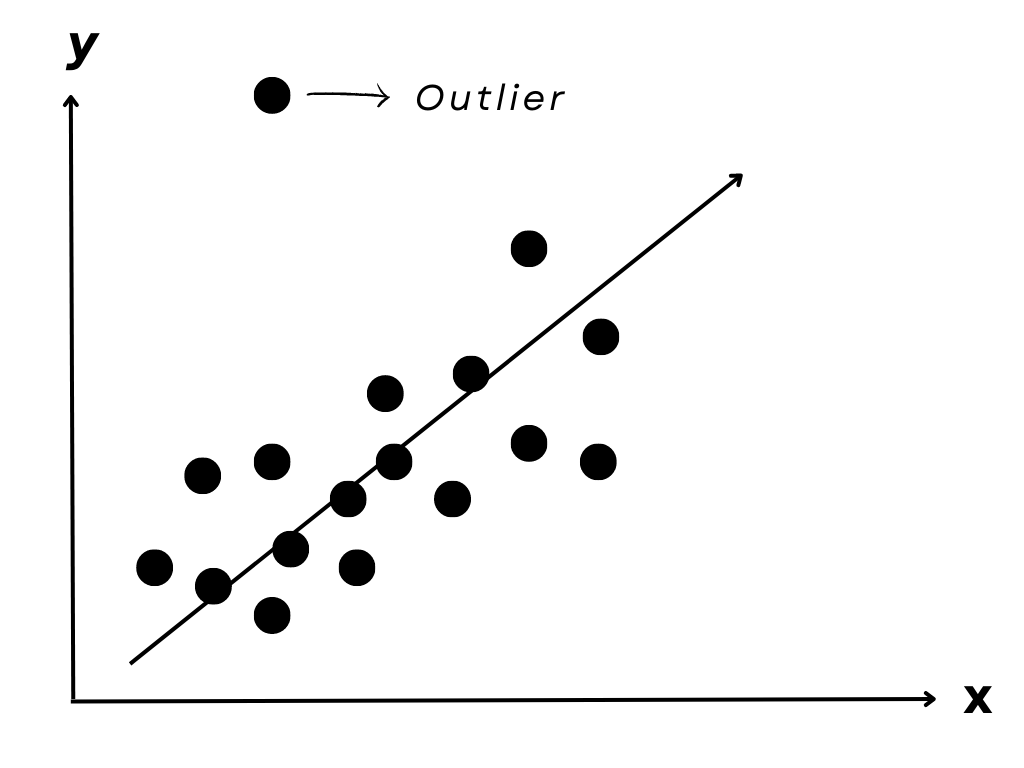
Outliers are extreme values that can skew statistical results.

Measurement errors, data entry errors, or other factors can cause them. Identifying and handling outliers appropriately in statistical analysis is vital to avoid inaccurate results.

In a normal distribution, outliers are typically defined as values that are more than 1.5 times the interquartile range (IQR) above the third quartile or below the first quartile.

Interquartile Range (IQR)

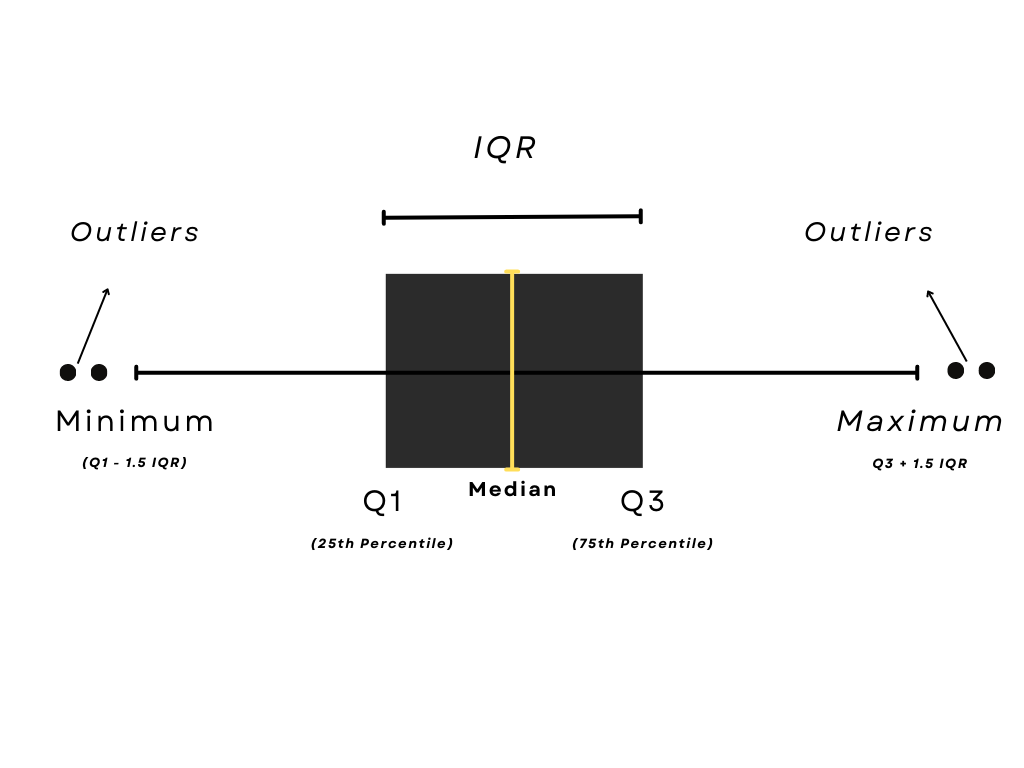
Interquartile Range in Statistics Cheat Sheet

The interquartile range or IQR is the difference between the third and first quartiles, which contains the middle 50% of the data.

Example: Assume a data set follows a normal distribution with a mean of 50 and a standard deviation of 10. If the third quartile is 60 and the first quartile is 40, then the IQR is 20.

Any value that is more than 1.5 times this IQR above the third quartile (i.e., more than 90) or below the first quartile (i.e., less than 10) would be considered an outlier.

Sampling

Sampling is the process of selecting a subset of a population to be analyzed in order to make inferences about the entire population.

Sampling methods can be probability-based or non-probability based.

Probability-based sampling refers to methods where each member of the population has a known probability of being selected.

The non-probability method is where the selection of individuals is based on convenience, judgment, or quota.

Example: Suppose a market research firm wants to estimate the average income of households in a city. They could select a random sample of households and collect income data from them. By analyzing the income data from the sample, they can make inferences about the average income of the entire population.

Normal Distribution

Normal distribution is a type of probability distribution that is commonly observed in real-world phenomena such as heights, weights, or IQ scores.

Due to its shape, it is also known as a Gaussian distribution or a bell curve.

A normal distribution's bell curve is defined by the mean and the standard deviation.

The mean is simply the average of the data points.

The standard deviation represents the degree of variability of the data.

The 68-95-99.7 rule is a useful tool for understanding the proportion of data that falls within different ranges of a normal distribution. According to this rule, 68% of the data are within one standard deviation of the mean, 95% are within two standard deviations of the mean, and 99.7% are within three standard deviations of the mean.

The 68-95-99.7 rule is used in many fields, including finance, engineering, and medicine, to help understand the variability and distribution of data.

By using this rule, we can predict the probability of a given event happening within a range of values and make informed decisions based on this.

Example: Imagine the mean height of a group of people is 5 feet 8 inches, and the standard deviation is 2 inches. The 68-95-99.7 rule estimates that approximately 68% of the group will have heights between 5 feet 6 inches and 5 feet 10 inches, approximately 95% will have heights between 5 feet 4 inches and 6 feet, and approximately 99.7% will have heights between 5 feet 2 inches and 6 feet 2 inches.

Confidence Intervals

A confidence interval suggests a range of values that is highly likely to contain a parameter of interest.

For example, suppose you sampled 5 customers who rated your product a mean of 3.5 out of 5 stars. You can use confidence intervals to determine what the population mean (the average rating of all customers) is based on this sample statistic.

Confidence Interval for means (n ≥ 30)

(\overline{x}\pm z\frac{\sigma}{\sqrt{n}})

Confidence Interval for means (n < 30)

(\overline{x}\pm t\frac{s}{\sqrt{n}})

Confidence Interval for proportions

(\hat{p}\pm z\sqrt{\frac{\hat{p}-(1-\hat{p})}{n}})

Hypothesis Testing

Hypothesis testing is used to determine how likely or unlikely a hypothesis is for a given sample of data. Technically, hypothesis testing is a method in which a sample dataset is compared against the population data.

Here are the steps to performing a hypothesis test:

State your null and alternative hypotheses. To reiterate, the null hypothesis typically states that everything is as normally was — that nothing has changed.
Set your significance level, the alpha. This is typically set at 5% but can be set at other levels depending on the situation and how severe it is to commit a type 1 and/or 2 error.
Collect sample data and calculate sample statistics (z-statistic or t-statistic)
Calculate the p-value given sample statistics. Once you get the sample statistics, you can determine the p-value through different methods. The most common methods are the T-score and Z-score for normal distributions.
Reject or do not reject the null hypothesis.

Example: Promotional Campaign

Statistics Cheat Sheet Promotional Campaign Example

Here is an example scenario of hypothesis testing.

A marketing team at a retail store is interested in determining whether a new promotional campaign has had a significant impact on sales.

They randomly selected two groups of customers: one group who saw the promotional ads and another who did not. They then record the sales from each group over the course of a week.

The hypothesis test can be performed as follows:

1. State the null and alternative hypotheses. The null hypothesis is that there is no difference in sales between the two groups of customers (i.e., the promotional campaign had no impact on sales). The alternative hypothesis is that there is a difference in sales between the two groups (i.e., the promotional campaign had a significant impact on sales).

H0:\mu1 = \mu2, H1:\mu1\neq \mu2

2. Set the significance level, alpha. Let's assume that the significance level is set at 0.05.

3. Collect the sample data and calculate the sample statistics. Let's say that the mean sales for the group who saw the promotional ads were $500, and the mean sales for those who did not were $450.

4. Calculate the p-value given the sample statistics. The p-value is the probability of obtaining a sample statistic as extreme or more extreme than the observed one, assuming that the null hypothesis is true. We can use a t-test or z-test depending on the sample size and distribution. Let's assume that we use a t-test with a two-tailed test.
The calculated t-value is:

t = \frac{500-450}{\sqrt{\frac{s_1^2}{n_1}+\frac{s_2^2}{n_2}}} = \frac{500-450}{\sqrt{\frac{50^2}{50}+\frac{30^2}{50}}}

where:
s1=50
n1=50
s2=30
n2=50

This yields a t-value of 6.06, with a corresponding p-value of 0.0001.

5. Reject or do not reject the null hypothesis. Since the p-value is less than the significance level (0.000000004 < 0.05), we reject the null hypothesis and conclude that there is enough evidence to suggest that the promotional campaign had a significant impact on sales.

This hypothesis test can help the marketing team make informed decisions about the effectiveness of their promotional campaign and potentially make adjustments to improve future campaigns.

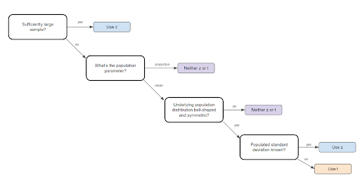
Z Statistic vs T Statistic

Z Statistics and T Statistics are important to know because they are required for step 3 in the steps to performing a hypothesis test (see above).

A Z-test is a hypothesis test with a normal distribution that uses a z-statistic. A z-test is used when you know the population variance or if you don’t know the population variance but have a large sample size.

Z = \frac{\bar{x}-\mu}{\frac{\sigma}{\sqrt{n}}}

A T-test is a hypothesis test with a t-distribution that uses a t-statistic. You would use a t-test when you don’t know the population variance and have a small sample size. You also need the degrees of freedom to convert a t-statistic to a p-value.

t=\frac{\overline{x}-\mu}{\frac{s}{\sqrt{n}}}

df = n-1

Example: Blood Pressure

Statistics Cheat Sheet Blood Pressure Example

Now let’s see how these statistics can be used in a real-life scenario.

A medical researcher wants to test whether a new drug is effective in reducing blood pressure in patients with hypertension.

They recruit a random sample of 30 patients with hypertension and measure their blood pressure before and after taking the drug.

To perform a hypothesis test on the drug's effectiveness, the researcher must determine whether the observed difference in blood pressure before and after taking medicine is statistically significant.

This involves calculating a test statistic, either a z-statistic or a t-statistic, and comparing it to a critical value or calculating a p-value.

If the population standard deviation is known, you can use a z-test to compare the mean blood pressure before and after taking the drug. The null hypothesis is that there is no difference in mean blood pressure before and after taking the medication, while the alternative hypothesis is that there is a difference.

If the population standard deviation is unknown, you must use a t-test. This is because the standard error of the mean must be estimated using the sample standard deviation, which will introduce additional variability into the test statistic. The t-test is more appropriate for small sample sizes, where the sample standard deviation is likely to be a poor estimate of the population standard deviation.

For example, let's say that the sample mean blood pressure before taking the drug is 150 mmHg, and the sample mean blood pressure after taking the drug is 140 mmHg, with a sample standard deviation of 10 mmHg.

The null hypothesis is that the mean difference is zero, and the alternative hypothesis is that the mean difference is less than zero (i.e., the drug effectively reduces blood pressure).

Z-Test

If the population standard deviation is known to be 10 mmHg, the researcher can use a z-test. The z-statistic is:

Z=\frac{\overline{x}-\mu}{\frac{\sigma}{\sqrt{n}}} = \frac{(140-150)}{\frac{10}{\sqrt{30}}} = -5.48

If the significance level is set at 0.05, the critical z-value for a one-tailed test is 1.645 (if it's a right-tailed test) or -1.645 (if it's a left-tailed test). Since it's a drug effectiveness study, we are likely interested in a decrease in blood pressure, which would make it a left-tailed test.

Therefore, the critical z-value is -1.645.

Since the calculated z-statistic is smaller (more negative) than the critical z-value, we reject the null hypothesis and conclude that the drug is effective in reducing blood pressure.

T-Test

If the population standard deviation is unknown, the researcher must use a t-test. The t-statistic is:

t = \frac{\overline{x}-\mu}{\frac{s}{\sqrt{n}}} = \frac{(140-150)}{\frac{10}{\sqrt{30}}} = -5.48

The result is the same as the z-value, as the population and sample standard deviation is the same in this example.

Using the t-distribution with 29 degrees of freedom and a significance level of 0.05, the critical t-value for a one-tailed test is 1.699. Since it's a drug effectiveness study, we are likely interested in a decrease in blood pressure, which would make it a left-tailed test.

Therefore, the critical t-value is -1.699.

Since the calculated t-statistic is smaller (more negative) than the critical t-value, we reject the null hypothesis and conclude that the drug is effective in reducing blood pressure.

This example shows how the choice between a z-test and a t-test depends on the known or estimated population standard deviation and the sample size. It also shows how these tests can be used in hypothesis testing to draw conclusions about the effectiveness of treatment.

A/B Testing

A/B testing in its simplest sense is an experiment on two variants to see which performs better based on a given metric. Technically speaking, A/B testing is a form of two-sample hypothesis testing, which is a method in determining whether the differences between two samples are statistically significant or not.

The steps to conducting an A/B test are exactly the same as a hypothesis test, except that the p-value is calculated differently depending on the type of A/B test.

An important aspect of A/B testing is choosing the right metric to measure the performance of the two variants. This metric should be relevant to the test goal, such as conversion rate, click-through rate, or revenue.

It's also essential to define the hypothesis before conducting the test, which involves specifying the null and alternative hypotheses and setting the significance level.

Another factor to consider in A/B testing is the sample size. The sample size should be large enough to detect a meaningful difference between the two variants while being small enough to keep the costs and time of the experiment manageable. The sample size calculation should take into account the expected effect size, the significance level, and the statistical power of the test.

A/B testing can be applied in many real-life situations.

Example: A software company may want to test two new feature versions to see which leads to more user engagement.

A fashion retailer may want to test two different product descriptions to see which one leads to more sales.

An e-commerce platform may want to test two different checkout processes to see which one leads to more completed orders.

In all of these cases, A/B testing can help determine which variant performs better and provide valuable insights for making data-driven decisions. By following the steps of hypothesis testing and using appropriate statistical tests, A/B testing can help businesses optimize their products, services, and marketing campaigns and ultimately improve their bottom line.

The type of A/B test that is conducted depends on a number of factors, which I’ll go over below:

Note: I won’t be covering the math behind these tests but feel free to check out Francesco’s article on A/B testing here.

Fisher’s Exact Test

The test was developed by Sir Ronald A. Fisher in the early 1900s and is used in various fields, such as genetics, social sciences, and marketing.

The Fisher’s test is used when testing against a discrete metric, like clickthrough rates (1 for yes, 0 for no). With a Fisher’s test, you can compute the exact p-value, but it is computationally expensive for large sample sizes.

Example: Advertising Campaign

Let's say you are a marketing researcher, and you want to know if a new advertising campaign effectively increases clickthrough rates on a website.

You randomly select two groups of website visitors. One group is shown the new ads, and the other is shown the old ones. You record the clickthrough rates for each group, i.e., the number of visitors who clicked on an ad divided by the total number of visitors in the group.

To test whether the new ads are more effective than the old ads, you can use Fisher's test.

This test will help you determine whether the difference in clickthrough rates between the two groups is statistically significant.

If the p-value is low enough (usually less than 0.05), you can conclude that the new ads are more effective in increasing clickthrough rates than the old ads.

Pearson’s Chi-squared Test

Chi-squared tests are an alternative to Fisher’s test when the sample size is too large. It is also used to test discrete metrics.

Example: Marketing Research

One real-life example of using Pearson's Chi-squared test is in the field of marketing research.

A company wants to determine if there is an association between a customer's age group (young, middle-aged, or elderly) and their preferred product category (food, clothing, or electronics).

They collect a random sample of 500 customers and record their age group and preferred product category.

To test for association, they use Pearson's Chi-squared test.

They create a contingency table with age group as the rows and product category as the columns. Then they calculate the expected frequencies assuming no association between the two variables.

They then compare the observed frequencies with the expected frequencies using the Chi-squared test statistic and calculate the p-value.

If the p-value is less than the significance level (e.g., 0.05), they reject the null hypothesis of no association and conclude that there is a significant association between a customer's age group and their preferred product category.

This information can be used by the company to tailor their marketing strategies to specific age groups and product categories.

Student’s t-test

I included the t-test and not the z-test because the z-test is typically impractical in reality since the population standard deviations are typically unknown. However, since we can get the sample standard deviation, a t-test is suitable.

It can be used under the conditions that the sample size is large (or the observations are normally distributed), and if the two samples have similar variances.

Example: Teaching Method Testing

Teaching Method Testing in Statistics Cheat Sheet

An example of using Student's t-test is a study where you want to compare the mean test scores of two groups of students who received different teaching methods.

The first group received traditional teaching methods. The second group received a new teaching method that the researchers hypothesized would lead to better test scores.

To conduct Student’s t-test, the researchers randomly assigned students to the two groups and administered the same test to both groups. They then calculated the sample mean and sample standard deviation for each group.

Since the population standard deviation was unknown and the sample size was small, they used Student's t-test. Student's t-test is a specific type of t-test that is commonly used for small sample sizes when the population variance is unknown. It helps you to find out whether the difference in means between the two groups was statistically significant or not, assuming the data are normally distributed and the two groups have similar variances.

By conducting the t-test, the researchers were able to determine whether the new teaching method was more effective than the traditional method in improving test scores.

Welch’s Test

Welch’s t-test is essentially the same thing as Student’s t-test except that it is used when the two samples do not have similar variances. In that case, Welch’s test can be used.

Example: Salary Testing

Salary Testing in Statistics Cheat Sheet

An example of using Welch's t-test is when a study wants to compare the salaries of two groups of employees in a company. One group is made up of managers and the other is made up of entry-level employees.

The researchers wanted to see if there was a significant difference in the average salary between the two groups.

However, the salaries of managers are typically more variable than entry-level employees, so the assumption of equal variances required for the Student's t-test was not met.

To address this, the researchers used Welch's t-test, which is appropriate when the two groups being compared have unequal variances.

This allowed them to determine whether there was a statistically significant difference in the average salary between the two groups, despite the unequal variances.

By conducting Welch's t-test, the researchers were able to determine if there was a significant salary gap between the two groups and take appropriate actions based on the findings.

Mann-Whitney U test

The Mann-Whitney test is a non-parametric test and should only be used when all assumptions for all previous tests are violated. For example, if you have a small sample size and the distributions are not normal, a Mann-Whitney test might be suitable.

Example: Medication Testing

Medication Testing in Statistics Cheat Sheet

An example of using the Mann-Whitney U test is in a study comparing the effectiveness of two different pain medications.

Suppose a small sample size is available, and the data collected is not normally distributed. In this case, the assumption for a t-test may not be met, and the Mann-Whitney U test could be used instead.

The researchers randomly assign patients to one of two groups to perform the test. The first group receives medication A, while the second group receives medication B.

The researchers then ask the patients to rate their pain on a scale of 1 to 10 after taking the medication. The scores are ranked from lowest to highest, and the test is conducted to determine if there is a significant difference in pain relief between the two medications.

The Mann-Whitney U test allows researchers to compare the effectiveness of two treatments without making assumptions about the normality of the data or the equality of variances between the groups.

To see how to conduct these tests in Python, check out this repository.

Cosine Similarity

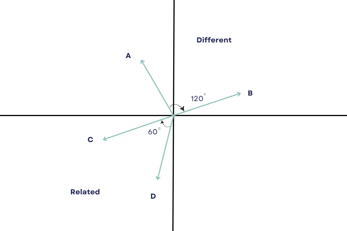
Cosine similarity is a way to measure how similar two sets of things are.

The more similar the two sets of things are, the closer they are to each other in this space.

The cosine similarity is calculated by looking at the angle between the two sets of things. If the angle is 0 degrees, that means they are exactly the same. If the angle is 90 degrees, that means they are completely different.

Example: Collaborative Filtering in Netflix

Collaborative filtering often uses cosine similarity to measure the similarity between items or users in a recommendation system.

By using cosine similarity to compare users or items, collaborative filtering can make recommendations based on the preferences of similar users or items.

A real-life example of collaborative filtering is the recommendation system used by Netflix. Netflix uses collaborative filtering to recommend movies and TV shows to its users based on their viewing history and the viewing history of similar users.

When a user watches a movie or TV show on Netflix, the system analyzes the user's viewing history. It compares it to the viewing histories of other users who have watched similar content. Based on the similarities between the viewing histories of different users, Netflix recommends other movies and TV shows that the user might enjoy.

For example, if a user has watched several action movies and TV shows, the collaborative filtering algorithm might recommend other action movies and TV shows to the user. Similarly, if several other users with similar viewing histories have enjoyed a particular movie or TV show, the algorithm might recommend that movie or TV show to the user.

By using collaborative filtering to make recommendations, Netflix can personalize its content for each individual user and provide them with a more enjoyable viewing experience.

Correlation

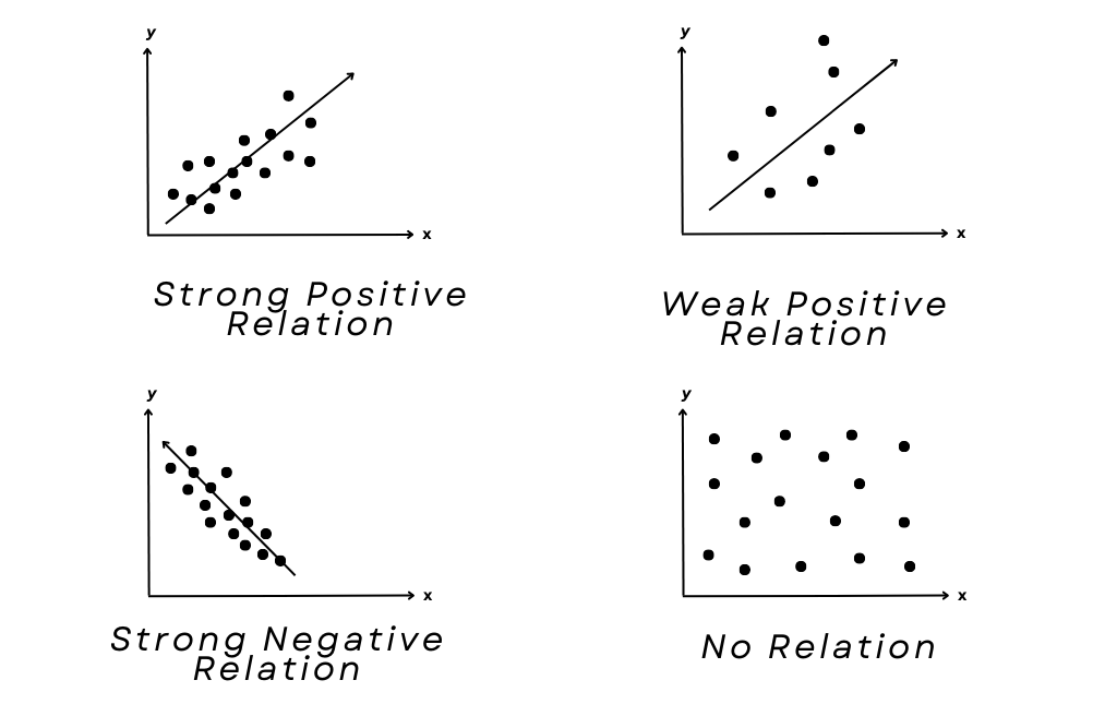
A statistical measure known as correlation analyzes the strength of the relationship or connection between two variables.

It ranges from -1 to 1.

A value of -1 indicates a perfect negative correlation.
A value of 0 indicates no correlation.
A value of 1 indicates a perfect positive correlation.

Correlation does not imply causation, but it can be used to identify potential relationships between variables.

Example: Suppose a researcher wants to investigate the relationship between the amount of exercise people do each week and their overall level of physical fitness. They could use a correlation coefficient to determine whether there is a significant relationship between these two variables.

Linear Regression

What is regression?

Regression is simply a statistical method for estimating the relationship between one or more independent variables (x) and a dependent variable (y). In simpler terms, it involves finding the ‘line of best fit’ that represents two or more variables.

The line of best fit is found by minimizing the squared distances between the points and the line of best fit — this is known as least squares regression. A residual is simply equal to the predicted value minus the actual value.

Residual analysis

A residual analysis can be conducted to assess the quality of a model, and also to identify outliers. A good model should have a homoscedastic residual plot, meaning that the error values are consistent overall.

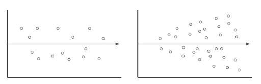
Homoscedastic plot (left) vs heteroscedastic plot (right)

Variable Selection

Two very simple and common approaches to variables selection are backward elimination (removing one variable at a time) or forward selection (adding one variable at a time).

You can assess whether a variable is significant in a model by calculating its p-value. Generally speaking, a good variable has a p-value of less than or equal to 0.05.

Model Evaluation

To evaluate a regression model, you can calculate its R-squared, which tells us how much of the variability in the data that the model accounts for. For example, if a model has an R-squared of 80%, then 80% of the variation in the data can be explained by the model.

The adjusted R-squared is a modified version of r-squared that adjusts for the number of predictors in the model; it increases if the new term improves the model more than would be expected by chance and vice versa.

3 Common pitfalls to avoid

Overfitting: Overfitting is an error where the model ‘fits’ the data too well, resulting in a model with high variance and low bias. As a consequence, an overfit model will inaccurately predict new data points even though it has a high accuracy on the training data. This typically happens when there are too many independent variables in the model.
Collinearity: This is when two independent variables in a model are correlated, which ultimately reduces the accuracy of the model.
Confounding variables: a confounding variable is a variable that isn’t included in the model but affects both the independent and dependent variables.

ANOVA (Analysis of Variance)

ANOVA is a statistical test used to analyze the differences between two or more groups of data.

It helps to determine whether the means of the groups are significantly different from each other or not.

The test compares the variance between the groups to the variance within the groups, and a significant result indicates that at least one group differs significantly from the others.

The formula for ANOVA is:

F = \frac{variance\ between\ groups}{variance\ within\ groups}

To evaluate the ANOVA score, you need to calculate the F-statistic and compare it to the critical value from an F-distribution table with a certain level of significance (alpha). Suppose the calculated F-statistic is greater than the critical value. In that case, you can reject the null hypothesis and conclude that there is a significant difference between at least two of the groups.

Example: Species Comparison

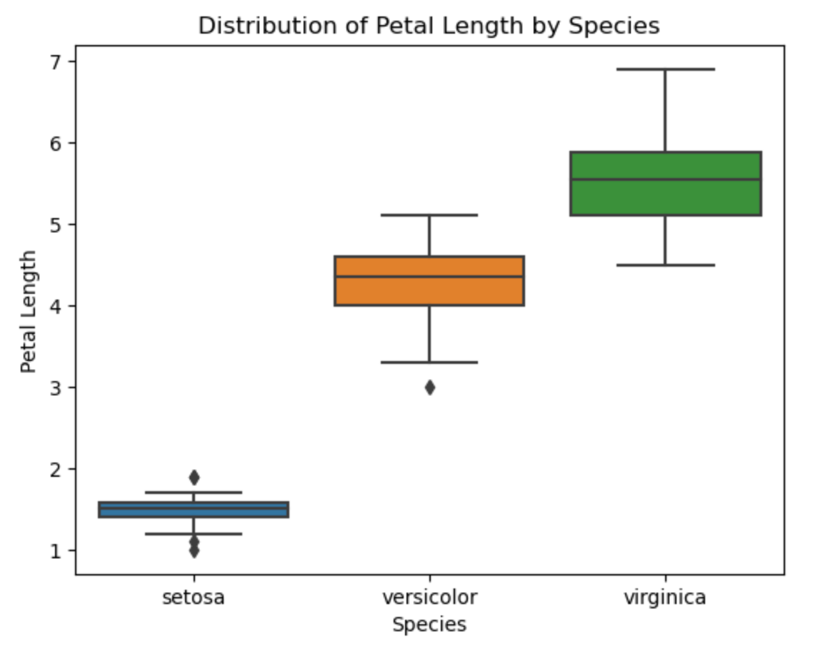
In this example, we performed an ANOVA test in Python to analyze the differences in the petal length of three different species of iris: setosa, versicolor, and virginica.

We first loaded the iris dataset using the seaborn library, which contains information about the petal length, width, and other variables for each species of iris.

We then separated each species' petal length data into three sets: setosa_petal_length, versicolor_petal_length, and virginica_petal_length.

We performed the ANOVA test using the f_oneway() function from the scipy.stats library. The test calculated the F-statistic and p-value for the analysis, which provided information about the statistical significance of the differences between the means of the petal length for the three species.

Here is the code.

from scipy.stats import f_oneway

# load the 'iris' dataset
iris = sns.load_dataset('iris')

# perform the ANOVA test
setosa_petal_length = iris[iris['species'] == 'setosa']['petal_length']
versicolor_petal_length = iris[iris['species'] == 'versicolor']['petal_length']
virginica_petal_length = iris[iris['species'] == 'virginica']['petal_length']

f_statistic, p_value = f_oneway(setosa_petal_length, versicolor_petal_length, virginica_petal_length)

# print the results
print('F-statistic:', f_statistic)
print('p-value:', p_value)

Here is the output.

The resulting F-statistic was 1180.16, which is a large value indicating that there is a significant difference between the means of the petal length for the three species.

The p-value was 2.86e-91, which is a very small value close to zero, indicating that the probability of observing such a large F-statistic by chance alone is very low.

Therefore, we can reject the null hypothesis that there is no significant difference between the three species' means of petal length. We conclude that there is a significant difference between the means of the petal length for at least one pair of species.

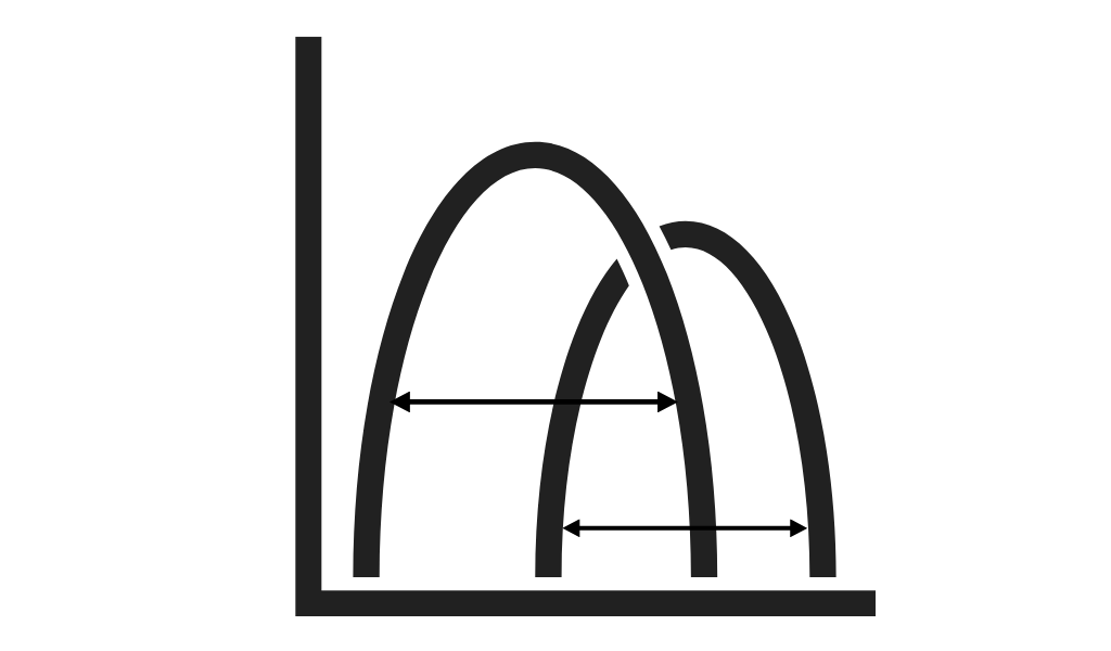
Central Limit Theorem

The central limit theorem states that if a random sample is drawn from any population, regardless of its distribution, the distribution of the sample means will be approximately normally distributed as the sample size increases.

Example: Coin Flip

Central Limit Theorem in Statistics Cheat Sheet

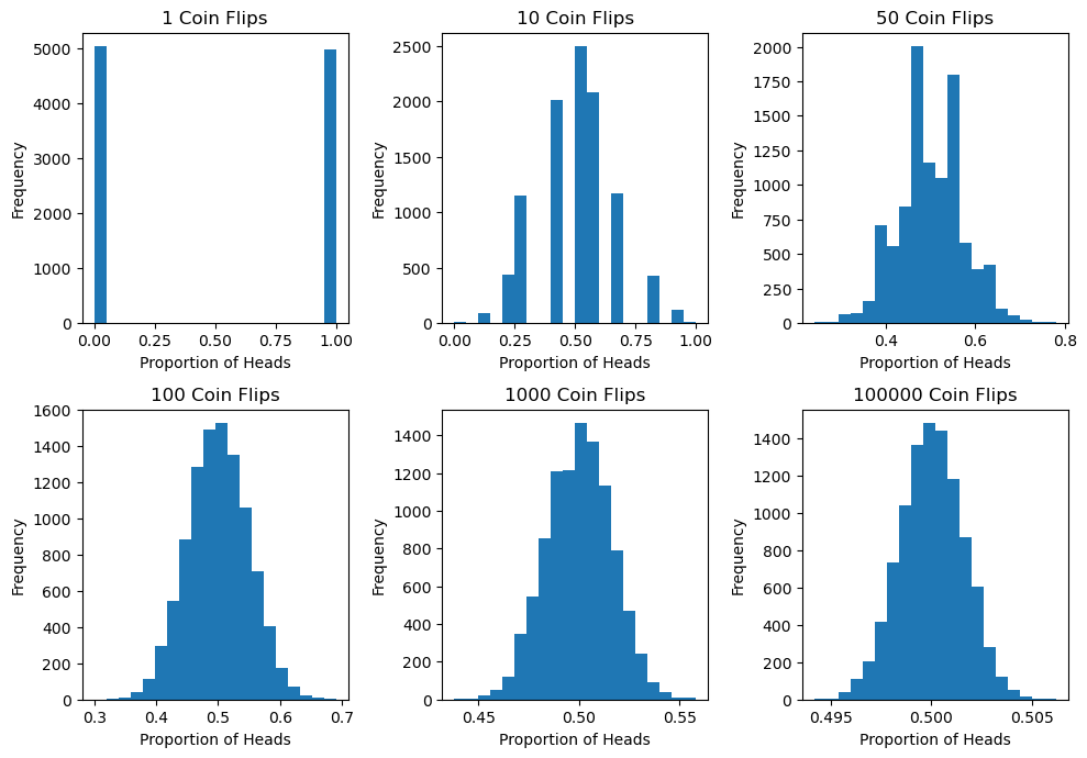
Suppose we flip a fair coin multiple times and record the number of times it lands heads up.

We repeat this process many times and record the average number of heads for each set of coin flips. In that case, the distribution of these averages will approximate a normal distribution as the number of coin flips increases.

For example, if we flip a coin once, the probability of getting heads might be one. If we flip the coin 10 times, the probability of getting heads will vary, which is not normally distributed.

However, if we repeat this process many times and record the average number of heads for each set of coin flips, the distribution of these averages will be approximately normal.

As we continue to increase the number of coin flips, the distribution of the sample means will continue to approach a normal distribution, as predicted by the central limit theorem.

This is a useful concept in statistics because it allows us to make inferences about a population based on a sample, even if we don't know the distribution of the population.

By using the central limit theorem, we can assume that the sample means will be normally distributed and use this information to perform hypothesis tests or construct confidence intervals.

Probability Rules

There are several fundamental properties and four probability rules that you should know. These probability rules serve as the foundation for more complex (but still fundamental) equations, like Bayes Theorem, which will be covered after.

Note: this does not review joint probability, union of events, or intersection of events. Review them beforehand if you do not know what these are.

Basic Properties

Every probability is between 0 and 1.
The sum of the probabilities of all possible outcomes equals 1.
If an event is impossible, it has a probability of 0.
Conversely, certain events have a probability of 1.

The Four Probability Rules

1. Addition Rule

The addition rule in probability says that if there are two events, A and B, which cannot happen at the same time, then the probability of either event happening is equal to the total of their probabilities.

This means that if the events are independent, we can add their probabilities to calculate the overall probability of either event happening.

Here is the formula.

P(A\ or\ B) = P(A) + P(B) - P(A\ and\ B)

P(A\cup B) = P(A) + P(B) - P(A\cap B)

Example: Consider a single toss of a fair coin. The probability of getting heads or tails is:

P(heads\ or\ tails) = \frac{1}{2} + \frac{1}{2} = 1

2. Complementary Rule

The complementary rule of probability says that when the probability of event A is represented by p, then the probability of event A not happening is represented by 1-p.

P(not\ A) = 1 - P(A)

P(\neg A) = 1 - P(A)

Example: The probability of getting a 2 on a standard six-sided die is 1/6. The probability of getting other than 2 is:

P(not\ 2) = 1 - \frac{1}{6} = \frac{5}{6}

3. Conditional Rule

Bayes theorem helps us calculate the conditional probability of the given events. Now let’s look at the formula and the example to make it clearer.

P(B\ given\ A) = \frac{P(A\ and\ B)}{P(A)}

P(B|A) = \frac{P(A\cap B)}{P(A)}

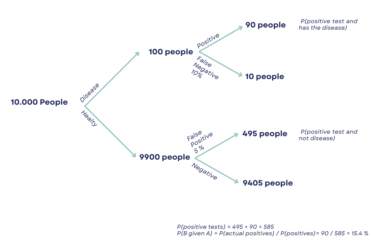
Example: A medical test for a certain disease has a false positive rate of 5% and a false negative rate of 10%. If 1% of the population has the disease, what is the probability that a person who tests positive actually has the disease?

Let’s explain this by giving numbers to these rates. We have a population of 10,000 people, and 1% or 100 people have the disease, while the other 9,900 do not.

Out of the 100 people who have the disease, 90 will test positive, and 10 will test negative.

Out of the 9,900 people who do not have the disease, 495 will test positive even though they do not have the disease, and 9,405 will test negative.

Using the formula

P(B\ given\ A) = \frac{P(A\ and\ B)}{P(A)}

we can calculate the probability that a person who tests positive actually has the disease as follows:

P(B given A) = P(positive test and has the disease) / P(positive test)

P(B\ given\ A) = \frac{P(positive\ test\ and\ has\ the\ disease)}{P(positive\ test)}

P(positive test and has the disease) = 90

P(positive\ test\ and\ has\ the\ disease) = 90

P(positive test) = (90 + 495) = 585

P(positive\ test) = (90+495) = 585

P(B given A) = 90 / 585 = approximately 0.154 or 15.4%

P(B\ given\ A) = \frac{90}{585} = 0.154 = 15.4\%

Therefore, the probability that a person who tests positive actually has the disease is approximately 15.4%.

4. Multiplication Rule

If events A and B are not related to each other, they are called independent events. In such cases, the probability of both events happening together is equal to the product of their individual probabilities.

P(A\ and\ B) = P(A)\cdot P(B\ given\ A)

P(A\cap B) = P(A)\cdot P(B|A)

Example: Let’s assume that you are drawing two cards from a standard deck of 52 cards. The probability of drawing an ace on the first draw is 4/52. The probability of drawing another ace on the second draw (assuming you did not replace the first card) is 3/51. The probability of drawing two aces is the product of these probabilities is:

P(A\ and\ B) = \frac{4}{52}\cdot \frac{3}{51} = \frac{1}{221}

To practice using these equations, you can check out this resource.

Bayes Theorem

Bayes theorem is a conditional probability statement, essentially it looks at the probability of one event (B) happening given that another event (A) has already happened. The formula is as follows:

P(A|B) = \frac{P(B|A)P(A)}{P(B)}

P(A) is the prior, which is the probability of A being true.
P(B|A) is the likelihood, the probability of B being true given A.
P(B) is the marginalization or the normalizing constant
P(A|B) is the posterior.

What you’ll find in a lot of practice problems is that the normalizing constant, P(B), is not given. In these cases, you can use the alternative version of Bayes Theorem, which is below:

P(A|B) = \frac{P(B|A)P(A)}{P(B|A)P(A)+P(B|\neg A)P(\neg A)}

To get a better understanding of Bayes Theorem and follow along with some practice questions, check out here.

Combinations and Permutations

Combinations and permutations are two slightly different ways that you can select objects from a set to form a subset. Permutations take into consideration the order of the subset whereas combinations do not.

Combinations and permutations are extremely important if you’re working on network security, pattern analysis, operations research, and more. Let’s review what each of the two are in further detail:

Permutations

Definition: A permutation of n elements is any arrangement of those n elements in a definite order. There are n factorial (n!) ways to arrange n elements. Note the bold: order matters!

The number of permutations of n things taken r-at-a-time is defined as the number of r-tuples that can be taken from n different elements and is equal to the following equation:

P_{n,r} = \frac{n!}{(n-r)!}

Example Question: How many permutations does a license plate have with 6 digits?

P_{9,6} = \frac{9!}{(9-6)!} = 60480

Combinations

Definition: The number of ways to choose r out of n objects where order doesn’t matter.

The number of combinations of n things taken r-at-a-time is defined as the number of subsets with r elements of a set with n elements and is equal to the following equation:

C_r^n = \frac{n!}{(n-r)!r!}

Example Question: How many ways can you draw 6 cards from a deck of 52 cards?

C_{6}^{52} = \frac{52!}{(52-6)!6!} = 20358520

Note that these are very very simple questions and that it can get much more complicated than this, but you should have a good idea of how it works with the examples above!

Summary

In this article, we covered all the important statistics concepts you’ll most likely get at any data science interview.

Statistics is one of the pillars of data science. There’s no serious data science project that doesn’t require the application of at least several statistics methods we discussed.

In real life, you’ll do statistical analysis, and build, train, and evaluate models in real life. Techniques available for sampling and hypothesis testing are crucial for these data science tasks, so no wonder they come up at the interviews very often.

To make the understanding easier, we backed up most of the theory with practical examples taken from experience in data science.