Machine Learning Algorithms Explained: Support Vector Machine

Brace yourself for a detailed explanation of the Support Vector Machine. You’ll learn everything you wanted and what you didn’t but really should know.

In this article, we’re going to deep dive into everything about the Support Vector Machine algorithm, starting from its concept and intuition up to the implementation example using the Scikit-learn library.

Specifically, here are some of the points that we will learn in this article:

• What a Support Vector Machine actually is
• Maximal margin Classifier
• Soft Margin and Support Vector Classifiers
• The intuition behind Support Vector Machine algorithm
• Support Vector Machine Under the Hood
• Support Vector Machine Implementation

So without further ado, let’s start with the first topic, which is the concept of what a Support Vector Machine algorithm actually is.

What is a Support Vector Machine?

Support Vector Machine (SVM) is one of the supervised machine learning algorithms that can be used for different purposes: classification, regression, and even anomaly detection. In a nutshell, the main focus of an SVM algorithm is to find the decision boundary that can separate different classes of data distinctively. Let’s use an example to make this point clearer.

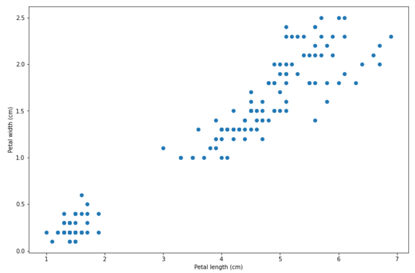
There are a lot of ways a decision boundary can be drawn in order to separate the data points above into two separate classes, as you can see below on the left-hand side:

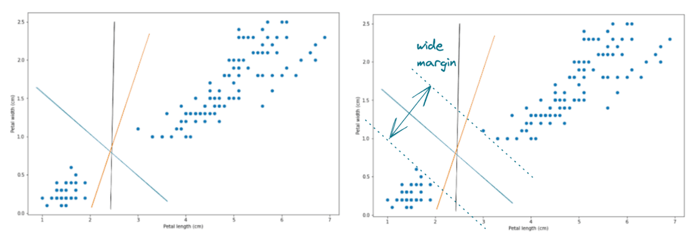
With all of the options above, the decision boundary in blue will be the most optimal one because of two things:

1. It provides a clear separation of data points into two different classes
2. More importantly, it also provides the largest margin between the decision boundary and the data points of each class that are located on the edge

And with the Support Vector Machine algorithm, in the end, we will end up with a decision boundary similar to the blue one above.

However, most of the time, the application of SVM is wrapped like a black box, in the sense that we implement it normally using a standardized library like Scikit-learn. This is all good, but it comes with a drawback: we don’t really know the decision logic behind the SVM algorithm.

In order to understand the logic behind the Support Vector Machine algorithm, let’s start with the concept of the Maximal Margin Classifier.

Maximal Margin Classifier

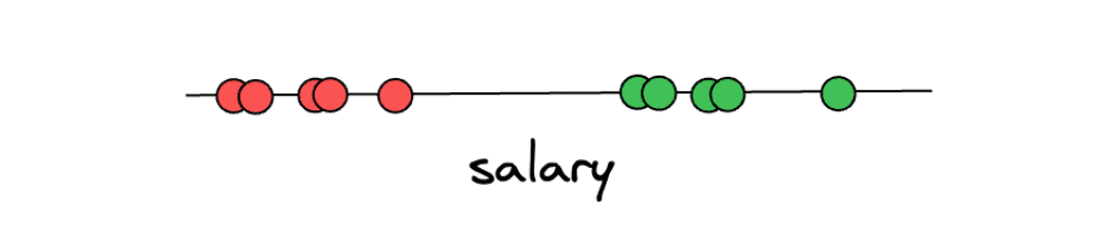
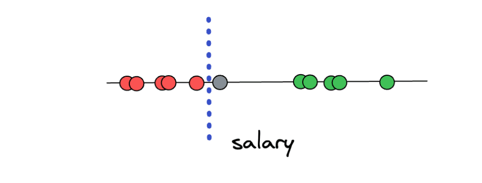
Let’s first imagine that we’re collecting data about people’s yearly salaries. After collecting the data on ten people’s yearly salaries, we label the data into two categories: either a person is underpaid or overpaid. In the example below, if a person is considered underpaid, then it will be labeled with red dots. Otherwise, if a person is considered overpaid, then it will be labeled with green dots.

From the above illustration, say we want to predict an unseen data point and determine whether that person is underpaid or overpaid. To do this, what we can do is create a threshold arbitrarily in-between two categories, as you can see in the illustration below:

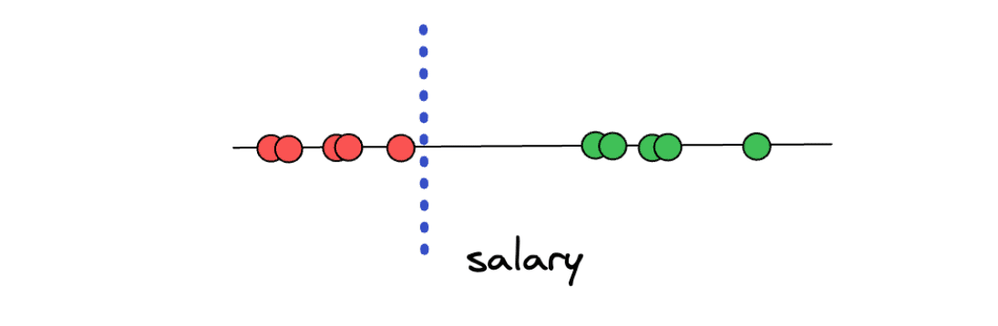
Now, with the threshold as above, we can easily classify a new unseen data point. If the new data point is above the threshold, then we can classify it as overpaid, and vice versa, if the new data point is below the threshold, then we can classify it as underpaid.

However, there is a big problem with this approach. What if we have a new data point that is located as shown in the illustration below?

Based on the threshold that we arbitrarily set in advance, this data point would be classified as overpaid. However, when we think about it, the prediction doesn’t make sense because this data point is closer to the ‘underpaid’ class compared to the ‘overpaid’ class. Thus, the method of setting an arbitrary threshold in-between two distinct classes is not the best solution.

So, now the question is, how can we improve this? How can we set a threshold such that the prediction of an unseen data point kinda makes sense?

One approach is to focus on the data points that are located on the edge of each of the distinct classes. Then, we create a threshold that has an equal distance to each of the data points that are located on the edge, as you can see in the following illustration:

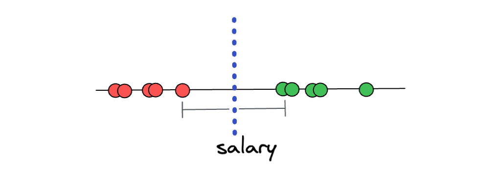
If the distance between the threshold and each of the edge points is equal, then we already find the widest margin possible, and this concept is called the Maximal Margin Classifier. With Maximal Margin Classifier, now the prediction of unseen data points would make sense due to the fact that if a new unseen data point is closer to the ‘overpaid’ class, it will be classified as ‘overpaid’, and vice versa.

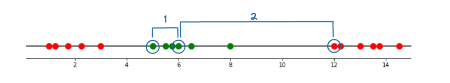
However, there is still one big problem with the Maximal Margin Classifiers concept. Can you imagine what will happen if we have an outlier in our data? As an example, let’s say we have the following data points:

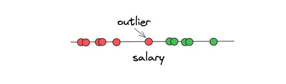
As you can see in the illustration above, one of ‘underpaid’ data points can be considered an outlier, as it deviates from the other ‘underpaid’ data points. The problem is, if we use the Maximal Margin Classifier concept, then we will end up with a threshold that looks something like this:

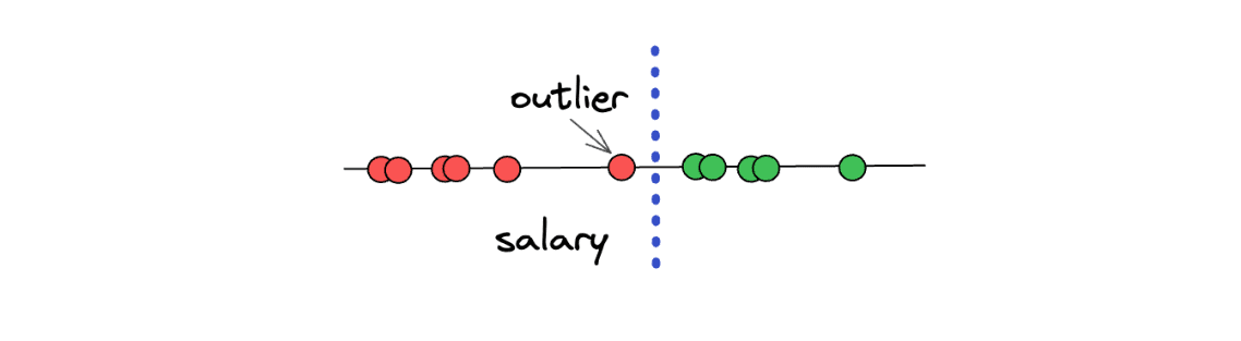
When we have an outlier in our dataset, then the concept of Maximal Margin Classifier will not work properly, and it will lead to a poor result. Thus, we can say that the Maximal Margin Classifier is very sensitive to the presence of outliers in a dataset. So, what can we do to improve the concept a little bit further to address the outliers? Let’s take a look at the concept behind Soft Margin.

Soft Margin and Support Vector Classifiers

The presence of outliers deteriorates the performance of Maximal Margin Classifiers, and what we can do to solve this problem is to deliberately allow some misclassifications to be made by our classifier.

Before we deep dive into this, let’s revisit the concept of Bias and Variance in Machine Learning.

• Bias measures the difference between the prediction’s mean value with the actual value of a point. If the difference is big, then we have a model with a high bias. This usually occurs when our model is too simple to capture the pattern of data points. In other words, our model underfits the data.
• Variance measures the spread of several predictions of a data point. The model with high variance usually occurs when it tries too hard to follow the pattern of each data point on our dataset, thus, it’s very sensitive to a small change in a data point. In other words, our model overfits the data.

To understand more about the difference between bias and variance, take a look at the following illustration:

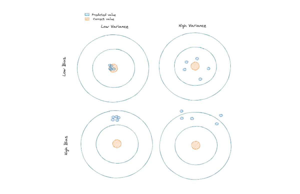
An ideal machine learning model would be one with low bias and low variance. However, this is often not realistic in practice, as we need to do some trade-offs between these two terms in order to come up with the optimal model. And this trade-off concept is also the one that we should use to improve Maximal Margin Classifiers.

Now that we know the theory behind bias and variance, the concept behind soft margin becomes easy to understand.

Soft margin extends the concept of Maximal Margin Classifiers by allowing the model to make misclassification and, thus, reducing its sensitivity to outliers. What we do with soft margin is basically to reduce the variance and increase the bias of Maximal Margin Classifiers. It might perform a little bit worse than before in fitting the data points, but we will get better performance when it tries to predict unseen data points.

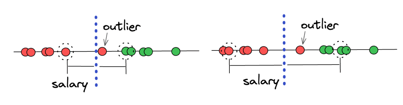
This now looks better, but you might want to ask: how do we choose which soft margin to use? In other words, how do we know whether the soft margin on the left-hand side is better than the soft margin on the right-hand side

Normally this is done using a cross-validation method, where the algorithm tries different varieties of soft margins to determine the number of misclassifications and data points that are allowed inside of it to get the best classification performance.

The data points on the edge of each soft margin are called Support Vectors. Hence, when we use the best soft margin in order to determine the threshold to classify data points, then this means that we use a method called Support Vector Classifiers.

However, even the soft margin method wouldn’t be a perfect method to use in a specific scenario. Let’s imagine we have the following data points.

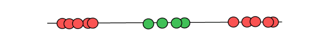
When we have a case as seen in the above illustration, it doesn’t matter what soft margin technique that we use and where our threshold classifier is, it will still misclassify a lot of data points. Clearly, relying solely on the soft margin concept itself wouldn’t be sufficient. And this is where we need a Support Vector Machine.

Intuition Behind Support Vector Machine

A Support Vector Machine (SVM) algorithm will solve our problem related to the case that we can see in the above illustration. In the simplest case, what an SVM algorithm does is it will calculate the relationship of one data point to another as if they are in the higher dimension.

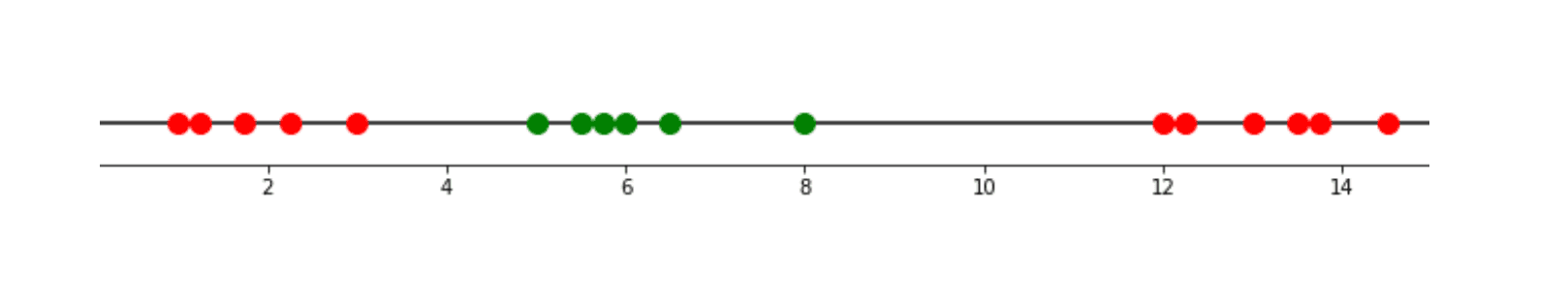
Take a look at the below example, we have basically a 1D dataset:

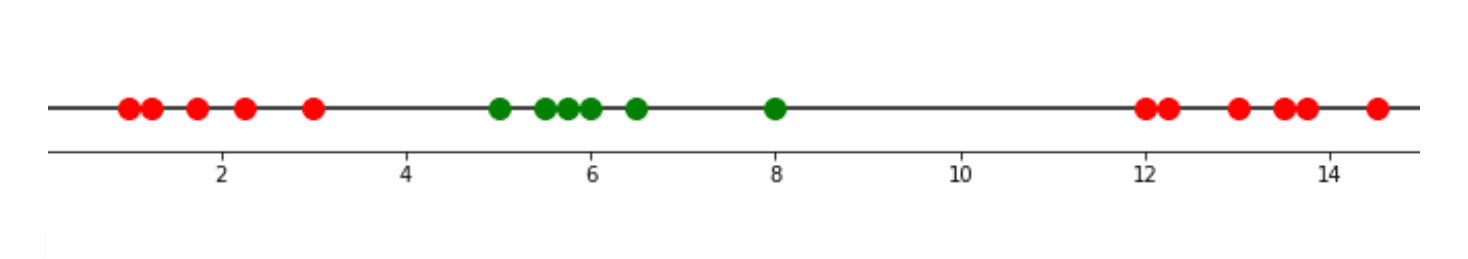
With an SVM algorithm, then it will do a so-called kernel trick, in which it will ‘transform’ our data into the higher dimension, let’s say, 2D, calculate the relationship between every pair of data points, and finally draw the Support Vector Classifier from there. Let’s take a look at how we can solve the problem above by doing this kernel trick.

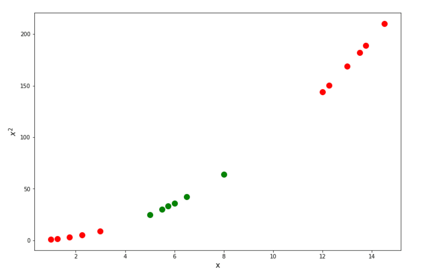
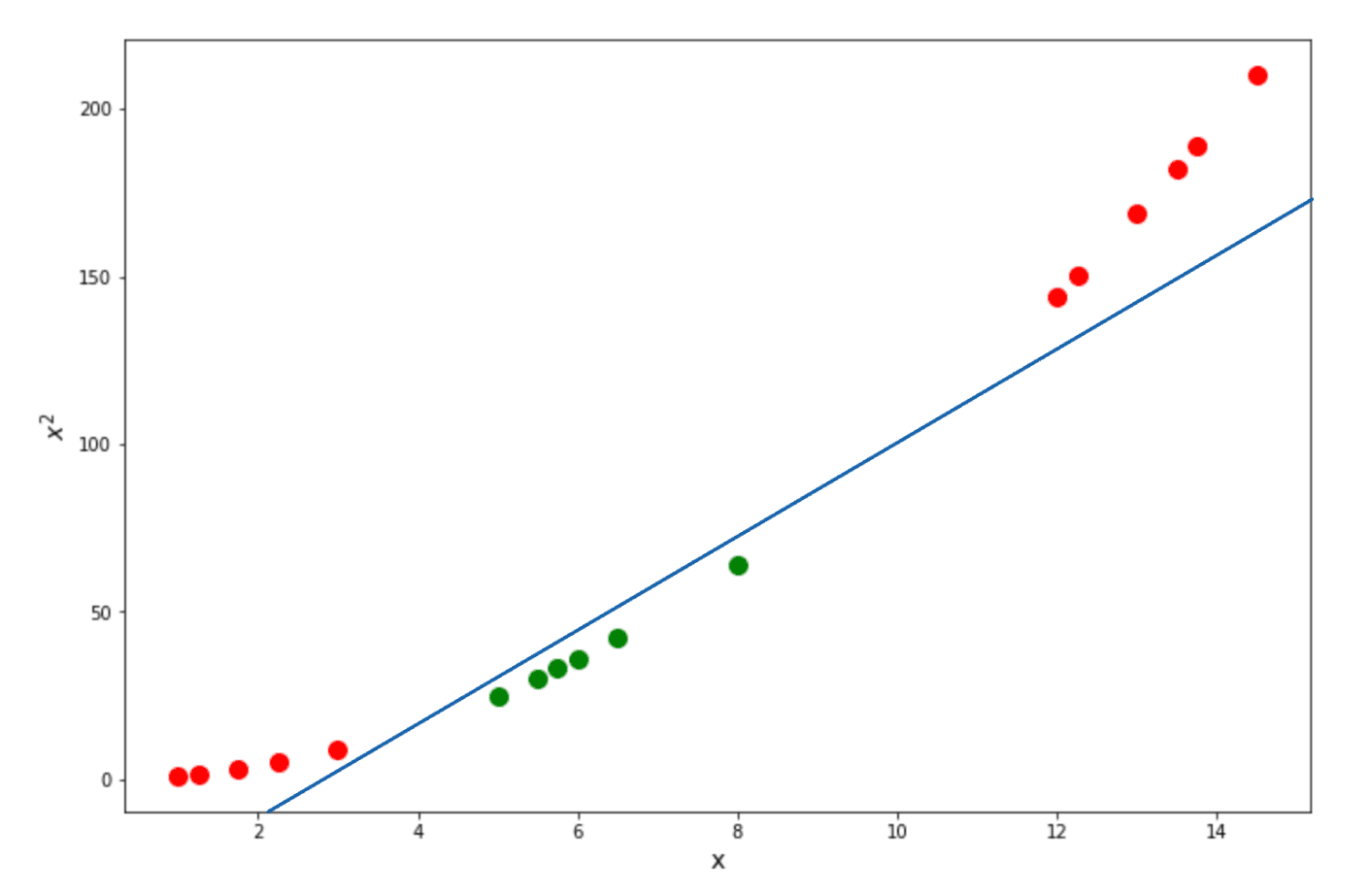
As you can see, when we try to calculate the relationship of our data in a higher dimension, then our data points become linearly separable, as we can draw the optimum Support Vector Classifier as follows:

Now the question is, why do we pick the square of our points on the Y-axis? Why not put a cubic representation of our points? Or even any other representation?

As mentioned above, an SVM algorithm uses the so-called kernel trick to treat our data points as if they are in a higher dimension. Thus, this kernel is the one that is responsible for how the algorithm represents the data in a higher dimension. The kernels that are commonly used in real-life applications, for example, linear kernel, polynomial kernel, and the so-called Radial Basis Function or RBF kernel.

To understand more about the concept of each kernel, let’s now deep dive into each of the kernels.

Polynomial Kernel

The SVM algorithm uses a kernel concept to calculate the relationship of our data points in a higher dimension, which can be in 2D, 3D, 4D, and so on. This concept is important because there might be a case that data points are not separable in a lower dimension, which leads to a poor fit in terms of the Support Vector Classifier.

Now, to calculate the relationship between a pair of data points, the polynomial kernel uses the following equation

where:
x: the first data point that needs to be compared
y: the second data point that needs to be compared
b: coefficient of the kernel
d: the polynomial degree

As you can see in the equation above, the d variable determines the degree of the polynomial, and to get the optimum number of coefficients, b, a cross-validation method is needed.

Now let’s use the equation above to derive and see what actually happens when we use the equation above to our data points. We’re going to use the same data points that you’ve already seen above:

Let’s say that we want to calculate the data points’ relationship with a polynomial degree of 2. After a cross-validation technique, let’s say we found out that the best coefficient of the kernel would be 0.5. Thus, we can plug these values into the equation as follows:

Since we have the polynomial degree of 2, then we can rewrite the above equation into:

Next, if we do the multiplication and then restructure the resulting equation, we will end up with the following equation:

And finally, we can decompose the above equation into our final form of the equation, as you can see below:

In the above equation, the x and y in the first position is basically the coordinate of two data points to be compared in the x-axis, and the square of that variable (the second position) is the coordinate of two data points in the y-axis, and the third position is the coordinate of two data points in the z-axis. Since we only have a polynomial degree of 2, then we can ignore the term in the third position, and we arrive at the following equation:

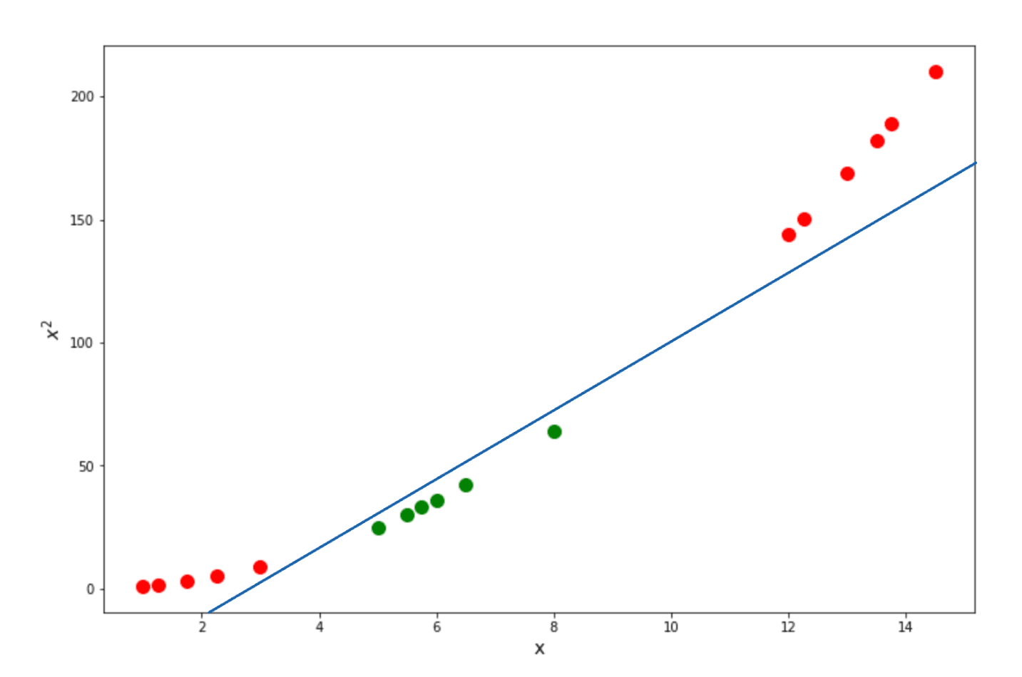
Finally we can calculate the relationship of data points in a higher dimension with the above equation. Below is the visualization of what our data points would be in 2D and how the Support Vector Classifiers can be drawn:

Now that we know the intuition behind the Polynomial kernel let’s take a look at another common kernel function used in Support Vector Machine, which is the Radial Basis Function kernel.

Radial Basis Function Kernel

If you know a supervised machine learning algorithm called k-Nearest Neighbors, then it will be quite simple to understand how this kernel trick works. In a nutshell, Radial Basis Function works similarly to the k-Nearest Neighbors algorithm in the sense that the closest neighbors of an unseen data point will have a big influence on how it will classify the unseen data point. Vice versa, the data points that are far away from our unseen data point will have little to no effect on our unseen data point.

The Radial Basis Function uses the following equation to determine the label of an unseen data point:

where:
x: the first data point to be compared
y: the second data point to be compared
γ: the scaling factor of the square distance between x and y

As you can see from the equation above, the relationship between any two particular data points is a function of squared distance, and the variable γ is the scaling factor of this squared distance function. Thus, we can say that γ is a variable that controls the influence of one data point on another. The optimal value of γ is normally determined via a cross-validation method.

So, let’s use the above equation to calculate the relationship in the two following scenarios:

1. Between two data points that are close to each other
2. Between two data points that are far from each other

To compute the scenario above, let’s assume that the γ value is equal to 1. In the first scenario, when we plug the value of two data points and compute the result, then we will get:

As you can see, we get the result of 0.36, now let’s calculate the second scenario:

When the two data points are located far away from each other, then we get a very small number, almost zero, which means that there is no relationship between the two data points. Meanwhile, if the two data points are located close to each other, then we get a result with a considerably higher value. It is important to notice that the value that we get in the end represents the relationship between a pair of data points in an infinite dimension.

Support Vector Machine Under the Hood

From the explanation about SVM in the previous sections, we now know that the big picture of a Support Vector Machine is to create a Support Vector Classifier with the widest margin from the edge of data points that belong to different classes with the help of a kernel trick. But you might be wondering, how is SVM able to generate the optimum Support Vector?

To answer this question, let’s take a look at the training process of a simple linear SVM classifier. In a nutshell, a linear SVM predicts an unseen data point, let’s call it x, by simply computing the following equation:

where:
w: the weights vector
b: bias term
x: unseen data point

If the result from that equation is positive, then it will be classified as 1, otherwise 0. During the training process of an SVM algorithm, we want to minimize the norm of weights vector w to maximize the margin. The smaller the w, the larger the margin that we’ll get.

Now to avoid any mistake in terms of a data point’s prediction, then the optimization of the Maximal Margin Classifier would be:

This means that we want the result of the equation to be greater than 1 for all positive data points (e.g., labeled as 1) and lower than -1 for all negative data (e.g., labeled as 0).

However, as we can see from the previous section, relying solely on Maximal Margin Classifiers alone in most cases wouldn’t be enough to obtain the optimal classifier. Thus, we need to add an additional constraint to introduce the soft margin concept. To do this, we introduce a new variable called a slack variable (ζ).

This slack variable controls the number of data points that are allowed to be inside of the support vectors. The introduction of this slack variable means that we have two contrasting objectives for our optimization process: on one side, we want to maximize the margin by minimizing the w, and on the other side, we want to make this slack variable as small as possible to keep the number of data points allowed inside of the support vector low.

Mathematically, we can describe the optimization process as follows:

If you take a look at the equation above, there is one new variable in our objective function, which is C. This is a hyperparameter that controls the trade-off between the objective function to obtain the best Maximal Margin Classifiers and the soft margin concept.

Support Vector Machine Implementation

As mentioned at the beginning of the article, the Support Vector Machine is a supervised machine learning algorithm that can be used for different tasks, such as regression, classification, and even for anomaly detection. In this section, we’re going to implement SVM in these three areas with Python and the scikit-learn library. So, let’s start with SVM implementation for classification use cases.

SVM for Classification

In a classification use case, our target variable (i.e., the variable that we want the machine learning model to predict) is either categorical or discrete. As an example, we want to predict whether an email is a spam or not, whether the animal in a picture is a cat or a dog, etc.

If we use SVM for classification problems, then its goal will be to create a Support Vector Classifier that maximizes the margins between data points with different classes, exactly as we have learned in the previous sections.

To use an SVM algorithm for a classification use case, let’s first create our data points.

from sklearn.datasets import make_blobs
import matplotlib.pyplot as plt

X, y = make_blobs(n_samples=40, centers=2, random_state=6)
y_green = y == 1
plt.figure(figsize=(12,8))
plt.scatter(X[~y_green][:, 0], X[~y_green][:, 1], color='red')
plt.scatter(X[y_green][:, 0], X[y_green][:, 1], color='green')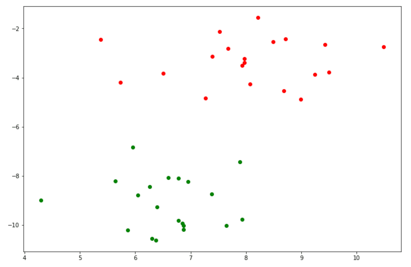

As you can see, now we have data points that consist of two different classes. To implement an SVM algorithm with Python, we can use the scikit-learn library to train the SVM on our data points.

from sklearn import svm

clf = svm.SVC(kernel="linear", C=1000)
clf.fit(X, y)

And that should be it. Now we can use our SVM model to predict the class of our data points and then visualize the decision boundary with the help of the matplotlib library.

from matplotlib import cm
from matplotlib.colors import ListedColormap,LinearSegmentedColormap
import numpy as np

hsv_modified = cm.get_cmap('hsv', 256)
newcmp = ListedColormap(hsv_modified(np.linspace(0.05, 0.4, 256)))

def make_meshgrid(x, y, h=.02):
   x_min, x_max = x.min() - 1, x.max() + 1
   y_min, y_max = y.min() - 1, y.max() + 1
   xx, yy = np.meshgrid(np.arange(x_min, x_max, h), np.arange(y_min, y_max, h))
   return xx, yy

def plot_contours(ax, clf, xx, yy, **params):
   Z = clf.predict(np.c_[xx.ravel(), yy.ravel()])
   Z = Z.reshape(xx.shape)
   out = ax.contourf(xx, yy, Z, cmap=newcmp, **params)
   return out

# plot the decision boundary

fig, ax = plt.subplots(figsize=(12,8))
# title for the plots
title = ('Decision boundary of linear SVC ')
# Set-up grid for plotting.
X0, X1 = X[:, 0], X[:, 1]
xx, yy = make_meshgrid(X0, X1)

plot_contours(ax, clf, xx, yy, alpha=0.15)
ax.scatter(X[~y_green][:, 0], X[~y_green][:, 1], color='red')
ax.scatter(X[y_green][:, 0], X[y_green][:, 1], color='green')
ax.set_ylabel('x')
ax.set_xlabel('y')
ax.set_xticks(())
ax.set_yticks(())
ax.set_title(title)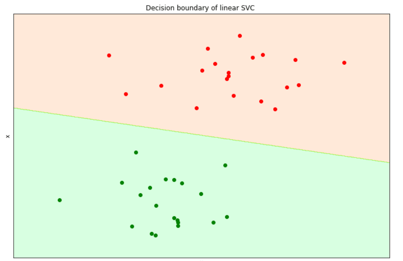

A linear SVM would be enough to solve the problem above as our data points are linearly separable, i.e., they can be separated via a straight line. But what if we have more complex data points as below?

from sklearn.datasets import make_moons

X, y = make_moons(noise=0.3, random_state=0)
y_green = y == 1
plt.figure(figsize=(12,8))
plt.scatter(X[~y_green][:, 0], X[~y_green][:, 1], color='red')
plt.scatter(X[y_green][:, 0], X[y_green][:, 1], color='green')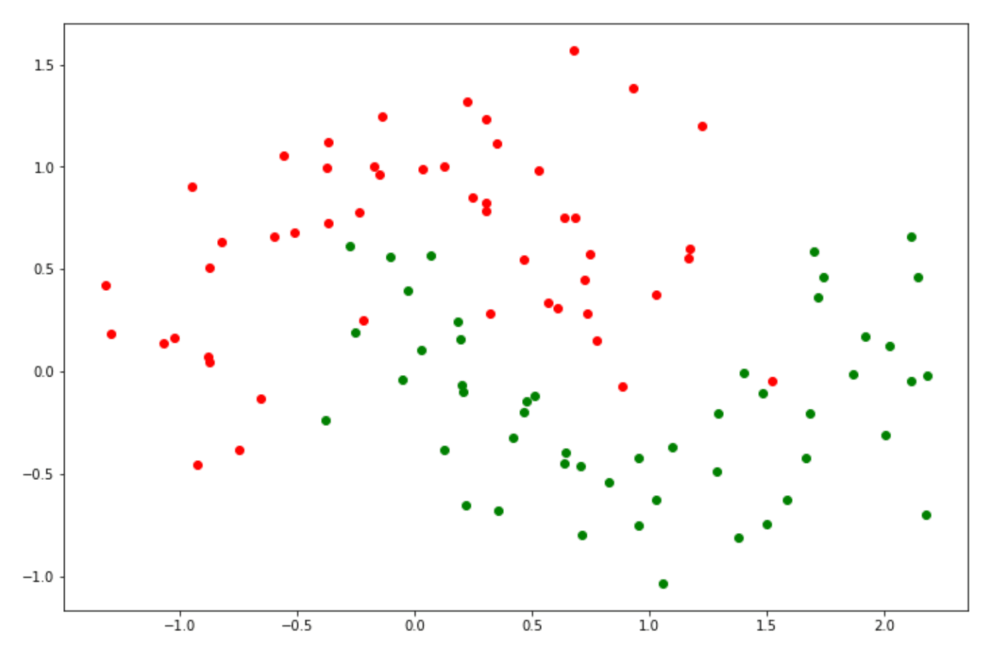

The data points above are not linearly separable, meaning that the algorithm can’t just create a simple straight Support Vector Classifier to separate between two classes. Thus, in this case, a linear SVM wouldn’t be the best option. In the previous sections, we mentioned that an SVM algorithm has the ability to calculate the relationship of data points in higher dimensions.

Thus, let’s try to solve this problem with a different kernel other than the linear kernel. Let’s use the Radial Basis Function kernel for this one to train the model, and then let’s plot the visualization of the decision boundary of the trained SVM model.

clf = svm.SVC(kernel="rbf")
clf.fit(X, y)

# plot the decision function

fig, ax = plt.subplots(figsize=(12,8))
# title for the plots
title = ('Decision boundary of RBF SVC ')
# Set-up grid for plotting.
X0, X1 = X[:, 0], X[:, 1]
xx, yy = make_meshgrid(X0, X1)

plot_contours(ax, clf, xx, yy, alpha=0.15)
ax.scatter(X[~y_green][:, 0], X[~y_green][:, 1], color='red')
ax.scatter(X[y_green][:, 0], X[y_green][:, 1], color='green')
ax.set_ylabel('x')
ax.set_xlabel('y')
ax.set_xticks(())
ax.set_yticks(())
ax.set_title(title)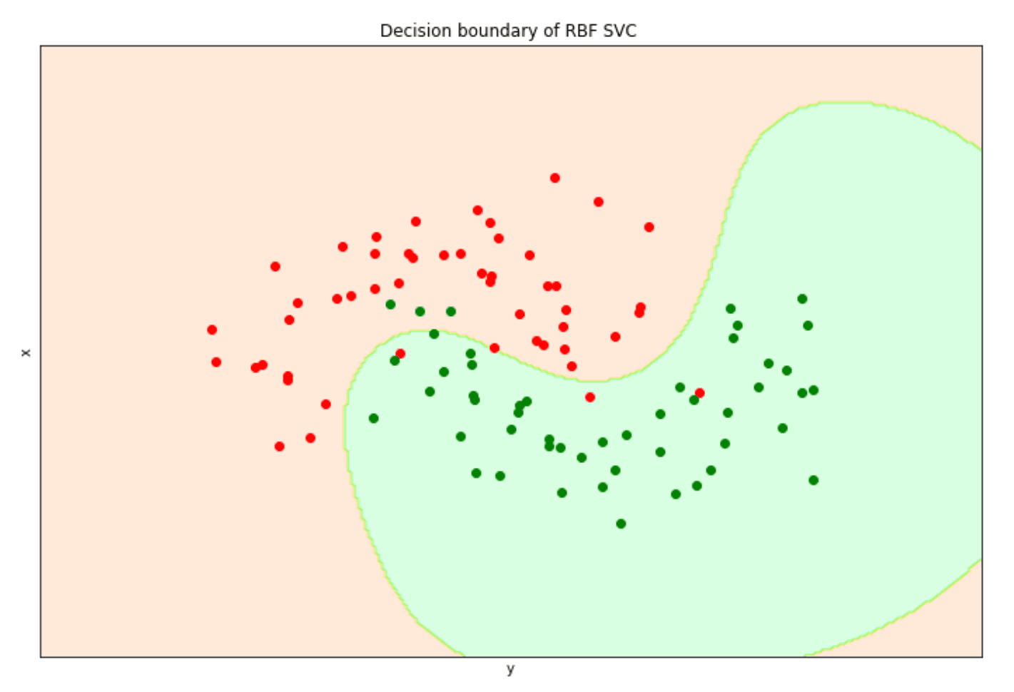

Although it’s not 100% perfect, the use of the Radial Basis Function kernel allows our SVM algorithm to create a non-linear decision boundary, as you can see in the visualization above.

SVM for Regression

Besides classification, SVM can also be useful as a regression machine learning algorithm. In a regression use case, the value that we want our SVM model to predict is continuous, such as the price of a house, a person’s weight, etc.

When we use SVM for regression use cases, the objective function of the algorithm is slightly different compared to classification purposes, in the sense that:

• In a classification problem, the goal of our SVM model is to create a Support Vector Classifier that maximizes the margin between two data points within two different classes.
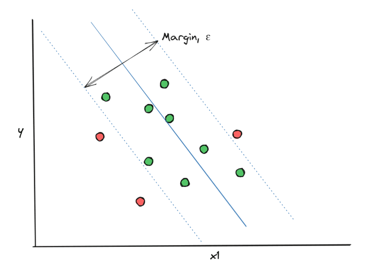
• In a regression problem, the goal of our SVM model is to create a Support Vector Classifier with a margin that fits as many data points as possible

In order to do this, first, we need to set in advance a hyperparameter ε, which is the maximum error allowed for our SVM algorithm to make. Next, the algorithm tries to fit a Support Vector Classifier that fits as many data points whilst also fulfilling the maximum error that we set in advance.

To implement an SVM algorithm for a regression problem, first let’s generate random data points with the help of the scikit-learn library.

from sklearn.datasets import make_regression
X, y = make_regression(
   n_samples=40, n_features=1, random_state=0, noise=8.0, bias=100.0)
plt.figure(figsize=(12,8))
plt.scatter(X, y, color='green')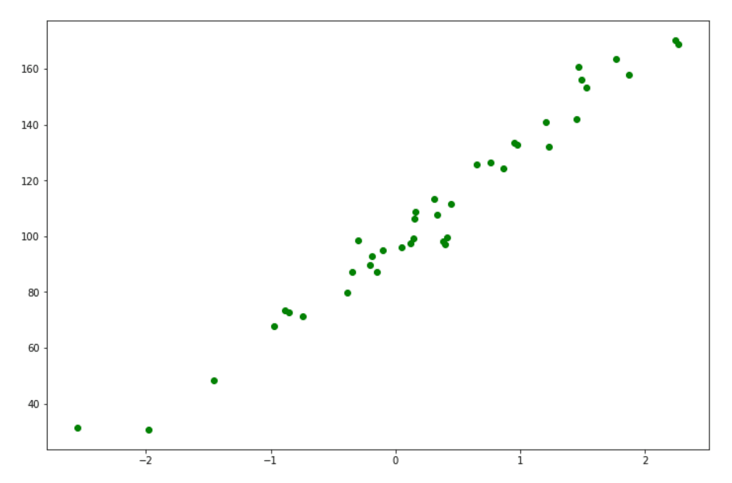

To implement SVM for a regression use case, we can use the SVR class from sklearn.SVM. Next, we can train the model on our data points above and then visualize the result.

from sklearn.svm import SVR
svr_lin = SVR(kernel="linear", C=100)
y_lin = svr_lin.fit(X,y).predict(X)

# Plot the result
lw = 0.5
plt.figure(figsize=(12,8))
plt.scatter(X, y, color='green')
plt.plot(X, y_lin, color='blue', lw=lw)
plt.xlabel('data')
plt.ylabel('target')
plt.title('Support Vector Regression')
plt.show()

As you can see, the problem that we have above is relatively simple, thus, a linear kernel would be sufficient to solve the problem. However, if we have more complex problems, just like what you can see below, the linear kernel would not be enough to arrive at the optimal solution.

X = np.sort(5 * np.random.rand(40, 1), axis=0)
y = np.sin(X).ravel()
y[::5] += 3 * (0.25 - np.random.rand(8))
plt.figure(figsize=(12,8))
plt.scatter(X, y, color='green')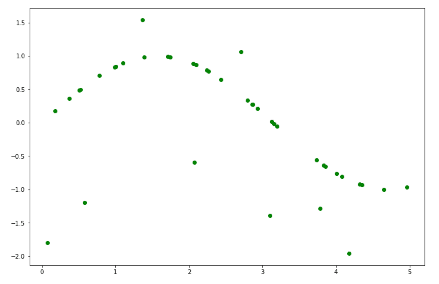

In this case, we need a more sophisticated kernel to solve the problem above. Thus, let’s use the Radial Basis Function kernel once again, train the model on the data points, and finally, let’s visualize the result.

svr_rbf = SVR(kernel="rbf", C=100)
y_rbf = svr_rbf.fit(X,y).predict(X)

# Plot the result
lw = 1
plt.figure(figsize=(12,8))
plt.scatter(X, y, color='green', label='data')
plt.plot(X, y_rbf, color='blue', lw=lw, label='Linear model')
plt.xlabel('data')
plt.ylabel('target')
plt.title('Support Vector Regression')
plt.show()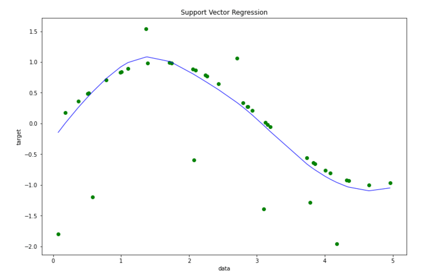

The Radial Basis Function kernel allows our SVM algorithm to learn a somewhat complicated pattern on our data points, which will be helpful to reduce the overall bias of the model.

Now that we know how to implement an SVM algorithm for regression problems, let’s move on to the next example of how the SVM algorithm could be useful, which is for anomaly detection.

SVM for Anomaly Detection

Anomaly detection is the term that refers to the process of identifying unusual patterns in our data. This process is widely used in many applications within our life, such as in the health sector, where anomaly detection algorithms assist the doctor in giving a more accurate diagnosis of the MRI scan result, etc.

There are a lot of anomaly detection algorithms out there that you can apply, and the SVM algorithm is one of them. The idea behind SVM as an anomaly detection algorithm is the use of the so-called one-Class SVM. In one-class SVM, the goal of the algorithm is to classify data points that consist of only one class instead of two or more, like we see normally in classification use cases. Thus, we can view one-class SVM as one of the unsupervised machine learning algorithms, as we don’t need to provide any label to our data points beforehand.

Since the algorithm has to classify data points that consist of only one class, then one possibility is that the resulting Support Vector Classifier would be in a circular shape. Thus, the goal is to fit the radius of the Support Vector Classifier with some optimization algorithms.

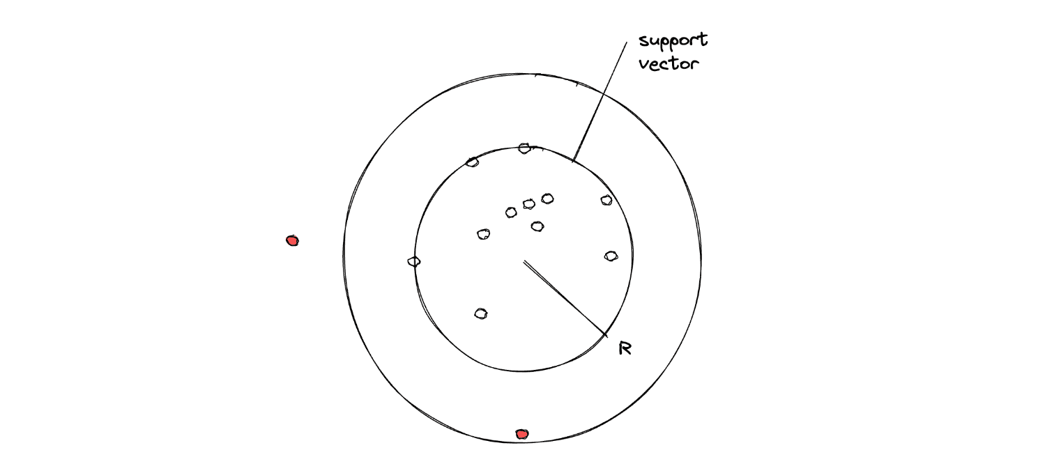
In the end, if there is a data point that lies outside of the radius of the optimized Support Vector, then that data point will be classified as an outlier.

We can indeed fine-tune the result of one-class SVM with a hyperparameter called nu (η) value. This hyperparameter controls the trade-off between the radius of the circle and the number of data points it can hold. In its implementation, η can take a value between 0 to 1, the smaller the value, the more data points that we try to fit in within the radius of the circle.

To implement one-class SVM with Python, we can use OneClassSVM class from the scikit-learn library. But before that, let’s generate random data points that we need to solve for an anomaly detection use case.

from sklearn.datasets import make_blobs

X, y_true = make_blobs(n_samples=100, centers=1, cluster_std=0.8, random_state=5)
X_append, y_true_append = make_blobs(n_samples=20,centers=1, cluster_std=5,random_state=5)

X = np.vstack([X,X_append])
y_true = np.hstack([y_true, [1 for _ in y_true_append]])

plt.figure(figsize=(12,9))
X = X[:, ::-1]
plt.scatter(X[:,0],X[:,1],marker="o", c='green');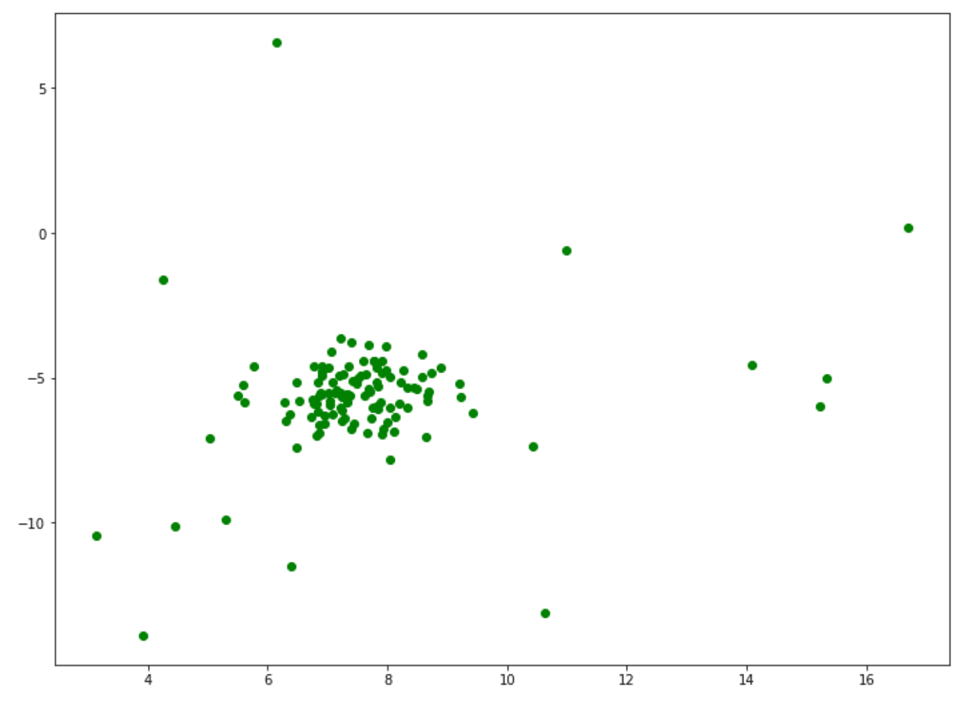

Next, let’s train our one-class SVM algorithm on the data points above and then visualize the result. In the following implementation, we set the η value to 0.1. If you’re not specifying it during model initialization, then the default value of 0.5 will be taken into account.

from sklearn.svm import OneClassSVM
one_svm = OneClassSVM(nu=0.1)
one_svm_label = one_svm.fit_predict(X)
index = np.where(one_svm_label == -1)
# Circling of anomalies
plt.figure(figsize=(12,9))
plt.scatter(X[:,0],X[:,1],marker="o", c='green');
plt.scatter(X[index,0],X[index,1],marker="o",facecolor="none",edgecolor="r",s=1000);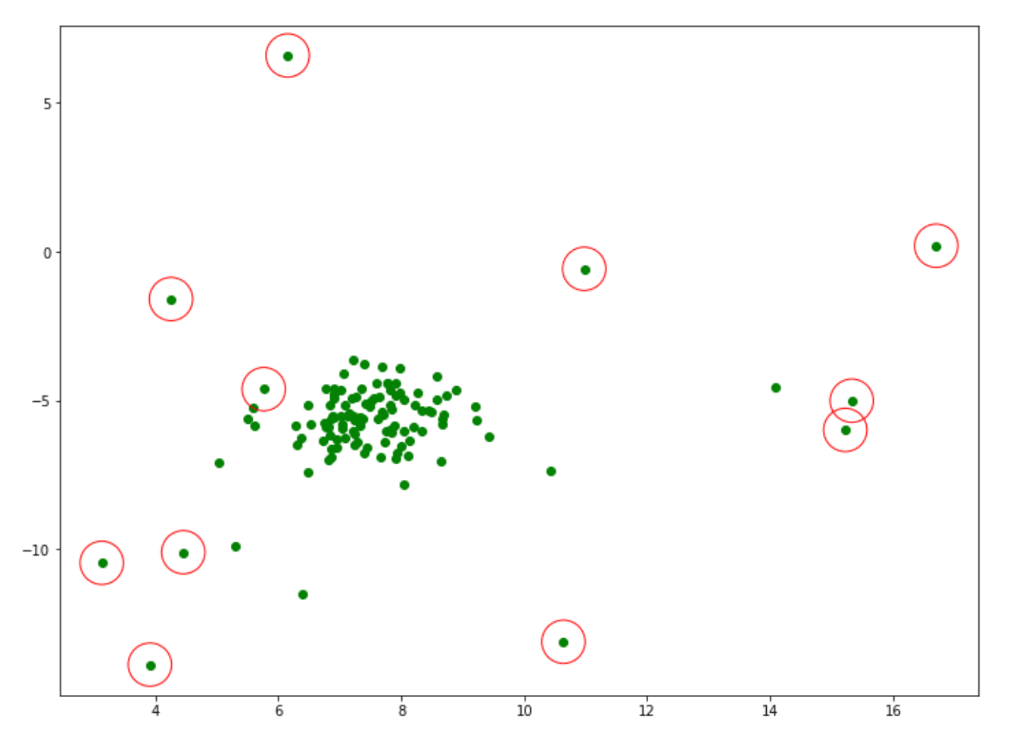

And that’s all we need to do! As you can see, the data points that are considered anomalies by our one-class SVM model are circled in red. To refine the result of the anomaly detection with one-class SVM, you can play around with the η value that we define during the model initialization.

Conclusion

In this article, we have learned a lot of things about the Support Vector Machine algorithm, starting from the concept of why we need it, the intuition behind it, to its implementation with Python.

Support Vector Machine is a supervised machine learning algorithm with high versatility, as we can use this algorithm for various cases, such as classifications, regression, or anomaly detections. In each case, we also have control to choose which kernel trick we want the algorithm to implement, which will help us to achieve better results in a somewhat complicated dataset.

If you want to learn more about other in-depth machine learning algorithm concepts, you can easily check out other StrataScratch articles, such as:

• If you want to learn about different kinds of clustering algorithms, check out this article  -> Machine Learning Clustering
• If you want to learn about the differences between supervised and unsupervised machine learning algorithms, check out this article -> Supervised vs Unsupervised Learning
• If you want to learn more about classification machine learning algorithms, check out this article -> Classification in Machine Learning