Overview of Machine Learning Algorithms: Classification

Let's discuss the most common use case "Classification algorithm" that you will find when dealing with machine learning.

Classification is arguably the most common use case that you will find when dealing with machine learning. A few examples of classification problems are:

• You want to build a model to predict if an email is spam or not
• You want to build a model to predict if that user comment that you just saw online has a positive or negative sentiment
• You want to build a model to predict if it’s an image of a dog or a cat

From a few use cases above, you might notice straight away that there is one particular thing in common when dealing with classification problems: the output is not a continuous value, but it’s a discrete value. The output will always be either a dog or a cat, either spam or not spam, either positive or negative, and no in-between.

Types of Classification Problems in Machine Learning

From the examples above, we now know that a particular characteristic of a classification problem is its output, where it has a discrete value instead of a continuous value.

To expand this concept a little bit further, there are three types of classification problems that you should know:

• Binary classification: the output only has two discrete values and we can only pick one of them, for example, cat or dog, spam or not spam, positive or negative, etc.
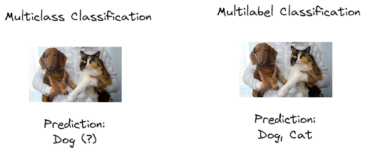
• Multi-class classification: the output has more than two discrete values and we can only pick one of them, for example {cat, dog, mouse, giraffe}, {positive, neutral, negative}, {very good, good, average, poor, very poor}, etc.
• Multi-label classification: the output has two or more discrete values and we can pick more than one of those values. Let’s say that we have an image that contains a dog and a cat in it. Instead of just predicting whether that image is an image of a cat or a dog, multi-label classification can output all both options.

Classification Algorithms in Machine Learning

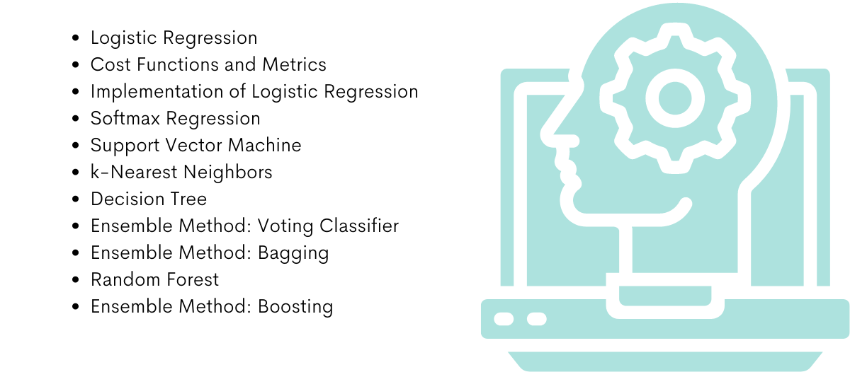
There are a lot of machine learning algorithms out there that we can use to solve classification problems, and we’re going to cover most of them in this article. In particular, here is the outline of classification algorithms in machine learning and what we’re going to learn in this article:

• Logistic Regression
• Cost Functions and Metrics
• Implementation of Logistic Regression
• Softmax Regression
• Support Vector Machine
• k-Nearest Neighbors
• Decision Tree
• Ensemble Method: Voting Classifier
• Ensemble Method: Bagging
• Random Forest
• Ensemble Method: Boosting

So without further ado, let’s start with the simplest of classification algorithms in machine learning, Logistic Regression.

Logistic Regression

If you have read the first article of this series about regression (which you can read here - Overview of Machine Learning Algorithms: Regression), you might be wondering if Logistic regression is actually a regression algorithm, due to the similar name with regression-based algorithms such as linear regression, Ridge regression, Lasso regression, etc. The answer is simple: it’s not.

The ‘regression’ word in Logistic regression refers to the similarity of mathematical formulation with the classical linear regression. This is because in Logistic regression, we still have a model that predicts the target variable y depending on the linear combination of predictors xi, same as in linear regression.

So, what differentiates Logistic regression from linear regression?

It’s the value of the target variable y. In linear regression, the target value y is a continuous value, ranging from minus infinity to plus infinity. Meanwhile, the target value is discrete in Logistic regression. Specifically, in a binary classification, the target value y has only two possible values, either 0 or 1.

Since we only have two possible values, then what we need as an output in Logistic regression is a value within a range of 0 to 1. To make sure that our output value has a range between 0 and 1, we need to use a Logistic function or commonly known as the sigmoid function.

which we can write in mathematical form as:

The sigmoid function above maps whatever output that we have at hand into a value within a range of 0 to 1. Thus, we have the so-called probability estimates, i.e we can imagine the output from the sigmoid function as a probability value, let’s call this value p.

If p is above a certain threshold, let’s say 0.5, then we can assume that our target value y has a value of 1 and vice versa, if p is below 0.5, then we can assume that target value y has a value of 0.

In case of Logistic regression, we have the following formula to approximate the probability estimates.

As you can see above, Logistic regression is similar to linear regression in the sense that it uses linear combinations of predictors. The difference is that in Logistic regression, we utilize the sigmoid function at the end to make sure that our output value is within a range of 0 to 1.

Now we know that how a Logistic regression generates an output, you might be wondering what the training steps of Logistic regression look like.

If we read the article about linear regression, we know about an approach called gradient descent to train a linear regression model. And gradient descent is also the approach that we use to train a Logistic regression model.

The only difference between training a linear regression and a Logistic regression is the cost function and the metrics that we use to train both models, i.e the goal that we want to achieve when we train them.

To train a linear regression model, we normally use a cost function and metrics such as Mean Squared Error (MSE), Root Mean Squared Error (RMSE), and Mean Absolute Error (MAE). However, in Logistic regression, we need to use different cost functions and metrics that we will discuss in the following section.

Classification Cost Functions and Metrics

As a quick introduction, there is a distinction between a cost function and a metric:

• Cost function is a value that we want to minimize during model training
• Metric is a value that we use to measure the goodness of prediction made by the model

In regression problems, normally we use the same value as a cost function and metric, i.e if we use MSE as the cost function, then we’re going to use MSE as well to measure the performance of the trained model. However, this is generally not the case in classification problems.

In general, we have to use a separate cost function and metric in classification problems due to an interpretability reason. We’re going to come back to this at the end of this section, but for now, let’s learn about cost functions and metrics commonly used in machine learning classification problems.

Cost Functions

As previously mentioned, a cost function refers to a value that we try to minimize during model training. And there is a specific difference in the minimization approach between regression and classification problems.

In a regression problem, the goal of the training process is to minimize the error between prediction and actual target value by squaring the residuals, i.e with the help of MSE, RMSE, or MAE. However, this is not the case in a classification problem, especially with Logistic regression.

With Logistic regression, our goal is to minimize the error between prediction and actual target value by maximizing the likelihood function. In general, the likelihood function has the following equation:

where p is the probability of data points coming up with a positive value (for example, an email is a spam) and 1-p is the probability of data points coming up with a negative value (for example, an email is not a spam).

In order to maximize the log-likelihood, we come up with a cross-entropy loss function as follows:

The main goal of cost function above is to make sure that we assign a high probability when the target value is 1, and assign a low probability value when the target value is 0.

If we think about it, this cost function makes sense because:

- If our target value is 1, then we end up with the following equation:

As the assigned probability p approaches 1, the lower -log(p) will be.

- If our target value is 0, then we end up with the following equation:

As the assigned probability p approaches 0, the lower -log(1-p) will be.

To minimize the cross-entropy loss function above, we need to use a gradient descent algorithm that you can learn more about in the first article of this series about regression.

Now that we know the common cost function for logistic regression, let’s talk about different metrics that are commonly applied in machine learning classification problems.

Classification Metrics

You already know that we commonly use MSE, MAE, or RMSE as metrics for regression problems. However, these metrics are not the preferred methods for classification problems. Instead, we use common metrics that are more intuitive to understand to measure the goodness of our classification model.

So let’s start with the most famous metric for classification problems, the accuracy.

Accuracy

Accuracy can be described as the ratio of the number of correct predictions with respect to the total number of samples, as you can see in the following equation:

As an example, let’s say that we have four data points. Out of those four, three data points are correctly predicted. Thus, we can put this into accuracy equation as follows:

Although it’s one of the most used metrics for classification problems, it has its weakness. Accuracy sometimes will fail to capture the true pattern in your data and will give you a false ‘promising’ result.

To illustrate this, let’s say that you have 100 data points. Out of those 100, 90 data points are labeled as 1 the other 10 are labeled as 0. Next, your model falsely predicted all of the data points that are labeled as 0. Hence, the model gives you a 90% accuracy score. It looks good on paper. However, we should know that this model is not good as it fails to predict even one single data point from class 0 correctly.

So, what are our other options? Let’s continue with the second metric.

Confusion Matrix

A confusion matrix gives us a summary of how good our classification model is in predicting the actual value of our target variable in the form of a table.

Normally, a confusion matrix can be visualized as a table where we have the predicted value in one axis and the actual ground-truth value of our variable in another axis.

As an example, let’s say that we have 100 data points, with 90 data points are labeled as 1 and the other 10 are labeled as 0, and they are all correctly predicted by our model. With a confusion matrix, we will get a summary of our model prediction as follows:

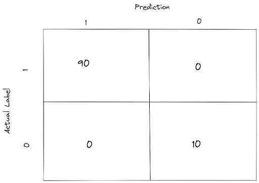
There are four terms in this confusion matrix that you should know to better understand the concept of metrics that we will talk about after this one.

• TP: True Positive; which means that our model predicts a data point as 1 when the actual label is 1 (good prediction).
• FP: False Positive; which means that our model predicts a data point as 1 when the actual label is 0 (bad prediction).
• TN: True Negative; which means that our model predicts a data point as 0 when the actual label is 0 (good prediction).
• FN: False Negative; which means that our model predicts a data point as 0 when the actual label is 1 (bad prediction).

Now that you know the concept of these terms, let’s continue to the next metric.

Precision and Recall

Precision can be described as the ratio of true positive with respect to the total number of positive predictions (true positive + false positive). Thus, we have the following precision equation:

Meanwhile, recall can be described as the ratio of true positive with respect to the total number of positive examples in our data points, i.e data points that are labeled as 1. Thus, we have the following equation for recall:

So, now the question is: which one is more preferred? Precision or recall?

It depends on your use case. Some use cases would demand our machine learning model to have high precision, and some would prefer a model with high recall value. In general, it’s impossible to have a model that has a high value in both precision and recall value. Often, we need to choose which metrics would be more suitable for our use case.

To illustrate this, let’s take a look at the following use cases:

• A spam detector. In a spam detector, it is better to classify spam email as legitimate (false negative) than classify a legitimate email as a spam (false positive). Thus, precision would be the better metric for this case.
• A cancer detector. In cancer detection, it’s better to diagnose cancer to a healthy person (false positive) than to diagnose that a person is healthy when he actually has cancer (false negative). Thus, the recall would be the better metric for this case.

Area Under the ROC Curve (AUC)

Before we learn how AUC works, we need to know what the ROC curve is first. ROC stands for Receiver Operating Characteristics and the curve consists of True Positive Rate (TPR) in one axis and False Positive Rate (FPR) in another axis.

TPR is defined exactly as Recall, i.e it has the same formula as you can see below:

Meanwhile, FPR can be described as the proportion of negative data points (labeled as 0) that are incorrectly predicted by the model. Thus, FPR has the following equation:

Both TPR and FPR has a range of value between 0 to 1. If we visualize RC curve, we get the following figure:

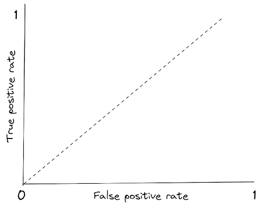
The dotted line represents the ROC curve of a random classifier. A good classification model will have a line that stays in the top left corner.

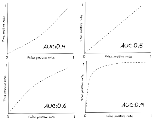
In general, the more the line stays towards the top-left corner, the larger the area under it, hence the higher the AUC score. Below is the visualization example of ROC curve with different AUC scores.

Now that we know common cost functions and metrics for classification algorithms in machine learning, let’s look back at the question: why should we use a different value for cost function and metrics? Why don’t we just use cross-entropy as the metric?

As mentioned before, it’s because of interpretability. Saying that a Logistic regression model has a cross-entropy of X on problem A and has a cross-entropy Y on problem B is difficult to interpret. It’s easier to say that a Logistic regression model has an accuracy of 90% on problem A and 75% on problem B.

So far, we already know about logistic regression and different kinds of metrics that we can use. Now it’s time for us to implement them. In the next section, we will use logistic regression to classify iris plant species and use each of the metrics mentioned above with Python.

About the Dataset

In this article, we’re going to use one dataset to demonstrate each classification algorithm in machine learning mentioned in the following sections. Hence, it’s better for us to get to know a little bit about the dataset that we’re working with.

We’re going to use the iris dataset in the entire article. Iris dataset consists of several predictors such as sepal length, sepal width, petal length, petal width, and the main goal is to identify the target variable that has 3 possible outcomes: Setosa, Versicolour, or Virginica.

Now let’s dive straight into the implementation of logistic regression.

Logistic Regression: Implementation

Implementing Logistic regression is very simple with the help of Python and scikit-learn library. We literally only need two lines of code to train a logistic regression with scikit-learn as follows:

from sklearn.linear_model import LogisticRegression

logistic = LogisticRegression()
logistic.fit(x, y)

Since at the moment we’re focusing on binary classification, let’s transform the dataset a little bit.

• Instead of trying to predict whether the target variable is Setosa, Versicolour, or Virginica, let’s transform it to Setosa and not Setosa. This way, we’re dealing with a binary classification problem instead of a multiclass classification.
• We use 80% of the data as training data and the other 20% as test data.
• For visualization purposes, let’s just use petal length as the only predictor.

Below is the complete implementation of building a logistic regression model in a binary classification problem with the iris dataset.

from sklearn import datasets
from sklearn.linear_model import LogisticRegression
from sklearn.model_selection import train_test_split

iris_data = datasets.load_iris()

X = iris_data.data[:, 2].reshape(-1,1)
y = (iris_data.target == 0).astype(np.int)#1 if Setosa, 0 anything else

X_train, X_test, y_train, y_test = train_test_split(X, y, test_size=0.2,random_state=42)

logistic = LogisticRegression()
logistic.fit(X_train, y_train)

And now we can visualize how Logistic regression makes a prediction based on petal length as follows:

x_new = np.linspace(0, 6, 1000).reshape(-1,1)
y_proba = logistic.predict_proba(x_new)

plt.figure(figsize=(12, 8))
plt.plot(x_new, y_proba[:, 1], 'g-', label='Setosa')
plt.plot(x_new, y_proba[:, 0], 'b--', label='not Setosa')
plt.xlabel('Petal length (cm)')
plt.ylabel('Probability')
plt.legend(loc="best")

As you can see from the decision boundary drawn from our Logistic regression model above, the probability that a flower is Setosa decreases as the petal length is increasing. Likewise, the probability that a flower is not a Setosa increase as the petal length is increasing.

For example, if our flower has a petal length that is shorter than 2 cm, our model is very certain that our flower is Setosa. Meanwhile, if our flower has a petal length longer than 4 cm, then our model is very certain that the flower is not Setosa. Our model becomes very uncertain when our flower has a petal length of 3 cm.

We’ve trained our Logistic regression model on our training data. Next, let’s assess its performance on the test data with each metric introduced in the previous section with scikit-learn as well.

from sklearn.metrics import accuracy_score, confusion_matrix, roc_curve, auc

acc = accuracy_score(y_test, logistic.predict(X_test))
conf_mat = confusion_matrix(y_test, logistic.predict(X_test))
fpr, tpr, thresholds = roc_curve(y_test, logistic.predict(X_test))
auc = auc(fpr, tpr)

print(f'Accuracy: {acc} | AUC: {auc}')
print('Confusion matrix:')
print(conf_mat)

# Output:
Accuracy: 1.0 | AUC: 1.0
Confusion matrix:
[[20  0]
[ 0 10]]

As you can see, our logistic regression performs perfectly well on the test set as it correctly predicts all of the test data. It has an accuracy of 1.0, an AUC of 1.0, and there is no False Positive or False Negative result as well.

So far, we’ve only considered the case where our target variable only has 2 possible outcomes (i.e binary classification: Setosa or not Setosa). However, what if the target variable has more than 2 possible outcomes?

Well, we can use softmax regression, which we will discuss in the next section.

Softmax Regression

Softmax regression is a generalization of Logistic regression to support multi-class classification in machine learning.

The idea is also more or less similar to the sigmoid function. Let’s say we have a data point x. Softmax regression will compute the probability score of data point x belongs to each class with the so-called softmax function.

The mathematical form of softmax function is:

where:

K: the number of classes
s(x): a vector that contains the score of each class for a data point x
f(s(x))k: the probability of a data point x belongs to each class

The optimization process of softmax regression is similar to Logistic regression, except that in softmax regression we sum over the total number of classes available.

Now let’s implement softmax regression in action with scikit-learn by going back to our iris dataset.

Previously with Logistic regression, we wanted to predict whether a flower is a Setosa or not Setosa, i.e there are only 2 classes. Now with softmax regression, we want to predict whether a flower is Setosa, Virginica, or Versicolour, i.e there are 3 classes. For visualization purposes, we are still going to use petal length as the only predictor.

We can implement softmax regression with scikit-learn as follows.

from sklearn import datasets
from sklearn.linear_model import LogisticRegression
from sklearn.model_selection import train_test_split

iris_data = datasets.load_iris()

X = iris_data.data[:, 2].reshape(-1,1) #For petal length
y = iris_data.target # All label considered

X_train, X_test, y_train, y_test = train_test_split(X, y, test_size=0.2,random_state=42)

softmax = LogisticRegression(multi_class= 'multinomial', solver='lbfgs')
softmax.fit(X_train, y_train)

Now after training our softmax regression model, we can use our model to predict an unseen data point. Let’s say that we have a flower with a petal length of 7 cm. We can feed this data into our model and it will return the probability of this data point belongs to each class, as you can see below:

print(softmax.predict_proba([[7]]))

#Output
array([[7.88035868e-09, 8.15289840e-04, 9.99184702e-01]])

As we can see above, our model assign a 99% probability on the third class for our data point, which means that our model is very certain that our data point is Virginica.

We can see the decision boundary drawn from our softmax regression model as follows:

x_new = np.linspace(0, 8, 1000).reshape(-1,1)
y_proba = softmax.predict_proba(x_new)

plt.figure(figsize=(12, 8))
plt.plot(x_new, y_proba[:, 0], 'g-', label='Setosa')
plt.plot(x_new, y_proba[:, 1], 'b-', label='Versicolour')
plt.plot(x_new, y_proba[:, 2], 'r-', label='Virginica')
plt.xlabel('Petal length (cm)')
plt.ylabel('Probability')
plt.legend(loc="best")

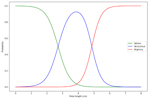
The interpretation of visualization above is similar to Logistic Regression:

• If our flower has a petal length below 2 cm, then our model is very certain that our flower is Setosa.
• If our flower has a petal length of around 4 cm, then our model is very certain that our flower is Versicolour.
• If our flower has a petal length above 6 cm, then our model is very certain that our flower is Virginica.

We can assess our model’s performance with accuracy and confusion matrix. Alternatively, if you prefer to assess your model with Precision and recall, you can do so with classification_report function from scikit-learn.

from sklearn.metrics import accuracy_score, confusion_matrix, classification_report

acc = accuracy_score(y_test, softmax.predict(X_test))
conf_mat = confusion_matrix(y_test, softmax.predict(X_test))
report = classification_report(y_test, softmax.predict(X_test))

print(f'Accuracy: {acc}')
print('Confusion matrix:')
print(conf_mat)
print('Classification report:')
print(report)

# Output

Accuracy: 1.0
Confusion matrix:
[[10  0  0]
 [ 0  9  0]
 [ 0  0 11]]
Classification report:
              precision    recall  f1-score   support

           0       1.00      1.00      1.00        10
           1       1.00      1.00      1.00         9
           2       1.00      1.00      1.00        11

    accuracy                           1.00        30
   macro avg       1.00      1.00      1.00        30
weighted avg       1.00      1.00      1.00        30

Support Vector Machines

Support Vector Machines (SVM) is a machine learning algorithm that can be used for both classification and regression tasks, but in this article we’re going to focus more on the classification side of it. To understand more how to use SVM for a regression task, refer to the regression series of this article.

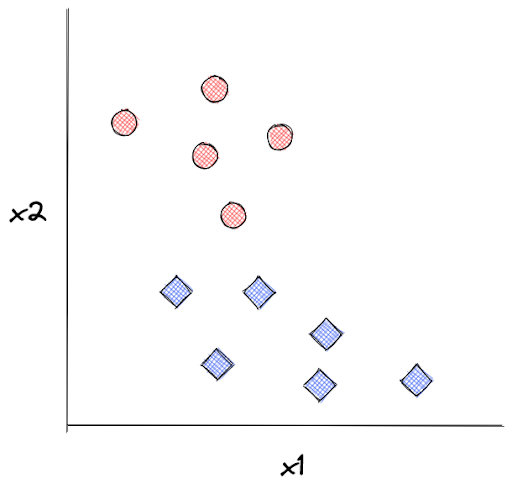
To understand how SVM works, let’s consider the data from our iris dataset. We’re going to visualize the data points of Setosa and Versicolor by their petal width and petal length, as you can see from the image below.

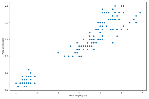
Now the question is, how does an SVM algorithm draw a decision boundary to separate between Setosa and Versicolor data points? There are several solutions for this, as you can see in the following images.

In order to create the optimum decision boundary, SVM uses a hyperplane with two margin lines. The main objective of SVM algorithm is to create a hyperplane with the widest possible margin lines.

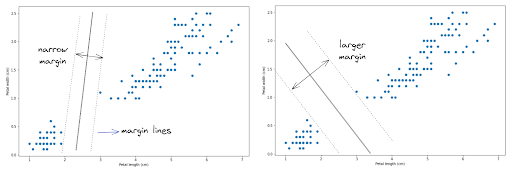
As you can see in the image above, there are a lot of different ways how a hyperplane can be drawn to create a decision boundary between data points. However, the main goal of SVM algorithm is to create a hyperplane with the widest possible margin lines to separate data points, as shown in the image on the right.

Implementation of SVM algorithm is made very simple with the help of scikit-learn library. Below is the example code on how to implement a linear SVM to predict whether a flower is Setosa or Versicolor.

from sklearn import datasets
from sklearn.preprocessing import StandardScaler
from sklearn.svm import SVC
from sklearn.pipeline import Pipeline
import numpy as np

iris_data = datasets.load_iris()

x = iris_data.data[:, 2:][0:100] #For petal length and petal width
y = np.asarray([i for i in iris_data.target if i == 0 or i == 1]).astype(np.float64)

svm_clf = Pipeline([
	('scaler', StandardScaler()),
	('linear_svc', SVC(kernel='linear'))
])

svm_clf.fit(x, y)

And below we can see the decision boundary of our linear SVM classifier:

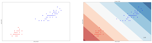
You might notice that in our case above, the data points are linearly separable, i.e we can draw a straight hyperplane to separate data points. However, this is normally not the case when we’re dealing with a more complex dataset. Sometimes the data points are not linearly separable, as can be seen in the following data points example.

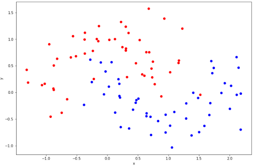
The data points above are not linearly separable, thus we can’t draw a straight hyperplane to separate the data points. Luckily, we can do classification for non-linear data points with SVM.

Let’s say that in our iris dataset, we use petal length (x1) and petal width (x2) as the predictors. The idea to do classification with non-linear data points is to transform the SVM function by adding additional predictors, which is the higher orders representation of our original predictors. To illustrate this, before we only have x1 and x2 as predictors, but after transformation, we have x1, x2, x3=(x12), and x4=(x22) as predictors.

With the help of scikit-learn, we can do the kernel trick to represent the illustration above by changing the kernel argument when we’re instantiating SVM class from ‘linear’ to ‘poly’, and then pick the polynomial degree that suits best our dataset, as you can see in the code snippet below.

svm_clf = Pipeline([
	('scaler', StandardScaler()),
	('poly_svc', SVC(kernel='poly', degree=3))
])

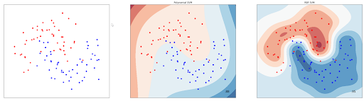
svm_clf.fit(x, y)

Aside of the polynomial kernel, we can also use the ‘‘RBF’ kernel to classify non-linear data points. Below is the example of a decision boundary drawn from the SVM algorithm with a 3rd-degree polynomial kernel and an RBF kernel:

One important thing to note when we try to implement SVM algorithm is that we need to scale our predictors. This is because SVM is very sensitive to feature scaling. Let’s say that we have two predictors, x1 and x2, and they have a very different scale: x1 is ranging from 1-10 and x2 is ranging from 1 to 100. If we left our predictors unscaled, then we will get the following hyperplane:

Now if we scale our predictors such that they have the same value range, we will get a much better hyperplane, as you can see below:

k-Nearest Neighbors (kNN)

k-nearest neighbors (kNN) is also one of the popular classification algorithms in machine learning. However, there is one fundamental concept that differentiates kNN from other classification algorithms in machine learning. Instead of removing all of the training data once the model has been built, kNN keeps all of the training data in the memory.

This is essential to explain how kNN works. Let’s say we have the following data points as our training data:

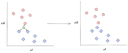
kNN algorithm will keep all of these data points such that when we supply the model with an unseen data point, let’s call it x, kNN can predict its label based on the distance between x with k number of its closest neighboring data points. Next, x will be assigned a label according to the label of the majority of its neighboring data points.

In the example below, the label of an unseen data point is assigned based on its 3 closest neighboring data points:

In order to detect which training data points that are the closest to x, kNN algorithm uses several metrics to measure the distance between x and its surrounding data points. Although there are many, but the most popular distance metric for kNN is the Euclidean distance, which has the following equation:

where:

x: the first data point
y: the second data point
d(x,y): the Euclidean distance between two data points

Aside of Euclidean distance, the most commonly used distance metrics applied in a kNN algorithm are the cosine similarity, Manhattan distance, Minkowski distance, and Chebyshev distance.

Same as SVM, kNN can be easily applied with the help of scikit-learn library. In the following code snippet, we’re going to use our iris dataset once again. Specifically, we’re trying to predict whether a flower is a Setosa or Versicolour based on its petal length and petal width.

from sklearn import datasets
from sklearn.preprocessing import StandardScaler
from sklearn.neighbors import KNeighborsClassifier
from sklearn.pipeline import Pipeline
import numpy as np

iris_data = datasets.load_iris()

x = iris_data.data[:, 2:][0:100] #For petal length and petal width
y = np.asarray([i for i in iris_data.target if i == 0 or i == 1]).astype(np.float64)

knn_clf = Pipeline([
	('scaler', StandardScaler()),
	('knn', KNeighborsClassifier(n_neighbors=3))
])

knn_clf.fit(x, y)

As you notice from the visualization of kNN’s decision boundary above, our iris dataset can be linearly separable which makes it easier for our kNN algorithm to assign the right label to an unseen data point. Now the question is, can kNN algorithm be used for nonlinear data points? The answer is yes.

To prove this, we can draw the decision boundary of kNN algorithm on non-linear data points presented in the SVM section above. The visualization below is drawn from a kNN algorithm that takes three closest neighbors into account:

Decision Tree

Decision Tree is arguably one of the most popular machine learning algorithms out there. Same as SVM, a decision tree can be used for both regression and classification tasks, although it’s more popular for a classification task.

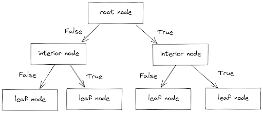
As the name suggests, a decision tree tries to classify the label of a data point by creating a bunch of branches consisting of interior nodes and leaf nodes.

• Interior nodes consist of conditions that each data point needs to fulfill
• Leaf nodes consist of the decision or label of each data point

In each branch, a data point will have to pass a series of boolean conditions, i.e True or False until it reaches a leaf node, which gives the final decision or label of that data point, as you can see below:

The natural question that comes after seeing the image above is, how does the decision tree algorithm decide the decision threshold in each branch?

To illustrate this, let’s get back to our iris dataset example. Let’s say that we want to classify the flower based on two features: petal length and petal width. The first objective of a decision tree algorithm is to split our training data points into two using a single predictor k and a threshold value of that predictor (i.e petal width > 16 cm).

But how does a decision tree algorithm pick which predictor to be used as a decider when in our case, we have two predictors (petal length and petal width)?

To do that, we need to train our decision tree classifier. The goal of this training process is to find the predictor and its corresponding threshold value that would be best to split our training data points into two. To determine the quality of splitting, we have the so-called Gini impurity as a common metric, which has the following equation:

where:

Gi: Gini impurity value
pi,k: ratio of class k among data points in the ith node

The lower the Gini impurity, the purer our subset is. This means that with a certain predictor and a certain threshold value, a perfect split of our training data points can be achieved (for example, the left branch consists of only Setosa and the right branch consists of only Versicolor.

The objective of the training process in a decision tree is to find the pair of predictor and threshold values that give us a low Gini impurity value, as you can see in the following cost function:

After it splits our training data into two, then it will try to split each subset of the new branch recursively using the same concept until it reaches the maximum depth of the tree specified in advance.

We can implement the decision tree algorithm easily with scikit-learn. To demonstrate this, we’re going to use our iris dataset again once more. In this example, we’re trying to classify
whether a flower is Setosa or Versicolor by using petal length and petal width as the predictors.

from sklearn import datasets
from sklearn.tree import DecisionTreeClassifier

iris_data = datasets.load_iris()

X = iris_data.data[:, 2:][0:100] #For petal length and petal width
y = np.asarray([i for i in iris_data.target if i == 0 or i == 1]).astype(np.float64)

tree_clf = DecisionTreeClassifier(max_depth=3)
tree_clf.fit(X, y)

Since the working concept of a decision tree algorithm can be easily interpreted, then we can visualize the decision process for each data point as follows:

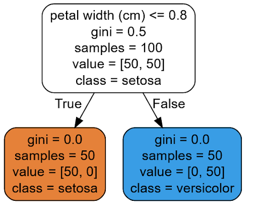
With the visualization above, we can easily follow the logic of how our Decision Tree model makes a prediction. As an example, let’s say that we have a new flower and we want this Decision Tree model to predict the class of our iris flower.

As a first step, our model will ask: is the petal width of our flower smaller or equal to 0.8? If yes, then the model predicts that our flower is Setosa and if not, it will predict that our model is Versicolour.

Next, as usual, we can also draw the decision boundary made by the Decision Tree and below is the visualization result of the decision boundary:

Decision Tree can also be used when our data is non-linear. To demonstrate how it performs on non-linear data points, we will use the same data from SVM and kNN sections. The decision boundary below is drawn by Decision Tree algorithm with the maximum depth equal to 3.

Ensemble Method: Voting Classifier

There are several methods out there to enhance the performance of machine learning algorithms to classify data points, and the ensemble method is one of them. Instead of using a single predictor to classify a data point, why don’t we use several classifier models to predict it? This is the idea behind ensemble method.

Let’s say that we have trained three machine learning models: a Logistic regression model, a Decision Tree model, and an SVM model on the same training data. Next, we want to predict an unseen data point and each of these models will predict the label of this data point.

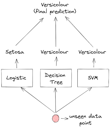
The prediction of each model will then be aggregated and the final prediction would be the one with the most votes. And this method is called voting classifier.

As you can see in the above visualization, if a Logistic regression model predicts that a flower is Setosa, but both Decision Tree and SVM model predict that a flower is Versicolour, then the final prediction will be Versicolour, because Versicolour got the most votes.

Implementing a voting classifier with scikit-learn is straightforward. In the following code snippet, we train three classifiers: a Decision Tree, a Logistic regression, and an SVM on our iris dataset. Then, we build a voting classifier on top of them to predict whether a flower is Setosa or Versicolour.

from sklearn.svm import SVC
from sklearn.tree import DecisionTreeClassifier
from sklearn.linear_model import LogisticRegression
from sklearn.model_selection import train_test_split
from sklearn import datasets
from sklearn.ensemble import VotingClassifier

X = iris_data.data[:, 2:][0:100] #For petal length and petal width
y = np.asarray([i for i in iris_data.target if i == 0 or i == 1]).astype(np.float64)

X_train, X_test, y_train, y_test = train_test_split(X, y, test_size=.4)

log_clf = LogisticRegression()
tree_clf = DecisionTreeClassifier()
svm_clf = SVC()

voting_clf = VotingClassifier(
    	estimators =[('lr', log_clf), ('tree', tree_clf), ('svc', svm_clf)],
    	voting='hard')

voting_clf.fit(X_train, y_train)

Next, let’s examine the performance of each model on test data and then compare their preformance with the voting classifier.

from sklearn.metrics import accuracy_score

for clf in (log_clf, tree_clf, svm_clf, voting_clf):
    
	clf.fit(X_train, y_train)
    
	y_pred = clf.predict(X_test)
	print(clf.__class__.__name__, accuracy_score(y_test, y_pred))

# Output:
LogisticRegression 1.0
DecisionTreeClassifier 1.0
SVC 1.0
VotingClassifier 1.0

As we can see above, the accuracy of all of the classifier is 1.0, hence it’s not surprising that the accuracy of the voting classifier is also 1.0. This is because the iris dataset is linearly separable and it’s easy for the classifier to classify an unseen data point.

Now let’s take a look at the performance of each classifier and the voting classifier on non-linear data points introduced in the previous section:

print(clf.__class__.__name__, accuracy_score(y_test, y_pred))

# Output

LogisticRegression 0.9
DecisionTreeClassifier 0.9
SVC 0.95
VotingClassifier 0.95

Most of the times, the accuracy of the voting classifier is equal or even better than the accuracy of each individual classifier.

There is a slight variation that you can try to tweak the voting classifier such that it will perform even better. As you might notice, we pass a parameter value ‘hard’ to variable ‘voting’ when we instantiate VotingClassifier class above. We can change it to ‘soft’ in order for the voting classifier to use soft voting instead of hard voting.

Soft voting means that instead of predicting a class of each data point based on the most-voted class, our classifiers will return a probability result that a data point belongs to each class, and then those probability values will be averaged and the class with the highest probability value will be selected as the class of our data point.

Below is the code snippet on how you can instantiate VotingClassifier with ‘soft’ voting:

voting_clf = VotingClassifier(
    	estimators =[('lr', log_clf), ('tree', tree_clf), ('svc', svm_clf)],
    	voting='soft')

Ensemble Method: Bagging

The second ensemble method that we’re going to learn is bagging. The big concept of bagging is similar to voting classifier, but instead of using a different set of classifiers, we are using the same classifier trained on a different subsets of our training data.

Now the question is: how does one classifier get a different subset of our training data?

This is normally can be achieved via random sampling, i.e we take a specific number of data points from a training instance randomly as samples, and then we use those samples to train our classifier model.

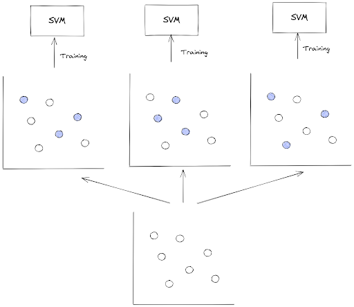
One important thing to note in bagging method is that the random sampling is performed with replacement or commonly called bootstrap in statistics. This means that a specific data point in a training instance can be selected more than once across different training processes of our classifier.

Once all classifiers are trained, then the ensembled model can make a prediction the same way as a voting classifier, i.e by aggregating the predictions from the classifiers.

We can implement bagging algorithm also with the help of scikit learn. Below is the example of how we can build and train a bagging classifier consists of several SVM models.

from sklearn.svm import SVC
from sklearn.ensemble import BaggingClassifier

bag_clf = BaggingClassifier(SVC(), n_estimators=100,
                       	max_samples= 10, bootstrap=True, n_jobs=-1)

bag_clf.fit(X_train, y_train)

Random Forest

Random Forest is one of the bagging-based classification algorithms in machine learning. It consists of several Decision Tree classifiers trained on a different subset of training data, as you can see in the visualization below.

There is a special class called RandomForestClassifier in scikit-learn that we can use to build and train a Random Forest model, as you can see in the code snippet below:

from sklearn.ensemble import RandomForestClassifier

rnd_clf = RandomForestClassifier(n_estimators=100, max_leaf_nodes = 3, n_jobs=-1)
rnd_clf.fit(X_train, y_train)

Same with Decision Tree classifier, Random Forests can also be used to classify data with non-linear data points. To demonstrate this, let’s take a look at how the decision boundary is drawn from Random Forests classifier on non-linear data points presented in Decision Tree section:

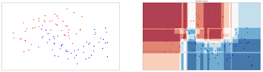
As you can see, Random Forest performs better on the same data in comparison with Decision Tree, as it achieves 95% accuracy compared to 93% accuracy with Decision Tree.

Another useful thing that we can do with Random Forest is feature importance inspection. This means that we can find out which predictors that play the highest part in affecting the prediction of our classifier. In our iris dataset, this could be either petal length, petal width, sepal length, or sepal width.

In order to do this, we can use feature_importances_method from RandomForestClassifier class from scikit-learn library, as you can see in the following code snippet.

from sklearn.ensemble import RandomForestClassifier
from sklearn import datasets

X = iris_data.data
y = iris_data.target

rnd_clf = RandomForestClassifier(max_depth=5, n_estimators=10, max_features=1)
rnd_clf.fit(X, y)

for name, score in zip(iris_data.feature_names, rnd_clf.feature_importances_):
	print(name, score)

# Output:
sepal length (cm) 0.19680743408033316
sepal width (cm) 0.08878813803715147
petal length (cm) 0.37398427810623264
petal width (cm) 0.3404201497762828

As we can see from the code snippet above, it turns out that petal length and petal width are the most important predictors for our Random Forest model to make a prediction compared to sepal length and sepal width.

Ensemble Method: Boosting

Another well-known ensemble method that is commonly applied in practice is Boosting. Boosting can be described as a method where we combine several weak classifiers and transform them into one strong classifier sequentially.

In this article of classification algorithms in machine learning, we’re going to focus more on two of the most commonly applied Boosting algorithms out there, which are AdaBoost and Gradient Boosting. So, let’s start with AdaBoost.

AdaBoost

AdaBoost converts several weak classifiers into one strong classifier by making sure that the next classifier will pay more attention to the data points that were underfitted by the previous classifier.

To make sure that the data points that were underfitted are going to get more attention by the next classifier, we change the weight of those data points and use the updated weights to train the next classifier.

To make the description above clearer, let’s take a look at the following visualization.

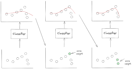
As you can see from the visualization above, AdaBoost transforms several weak classifiers into a strong classifier sequentially or step-by-step. This means that one classifier can only be trained after the previous classifier has been trained and evaluated.

This sequential nature of AdaBoost makes it impossible to parallelize the process during the training process. Thus, it doesn’t scale well if we have a lot of classifiers to combine.

As usual, we can implement AdaBoost easily with the help of scikit-learn library. Below is the code snippet on how we can build and train an AdaBoost model consisting of several Decision Tree classifiers.

from sklearn.ensemble import AdaBoostClassifier
from sklearn.tree import DecisionTreeClassifier

ada_clf = AdaBoostClassifier(DecisionTreeClassifier(max_depth=5), n_estimators=10, algorithm="SAMME.R")

ada_clf.fit(X_train, y_train)

AdaBoost can be applied to linearly separable data points and also to those that are not linearly separable. To demonstrate this, let’s visualize the boundary decision drawn by AdaBoost model on non-linear data points presented in the previous section. Below is the visualization of AdaBoost’s decision boundary.

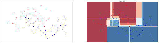
As we can see, it achieves an accuracy of 95% on these data points, pretty much comparable with Random Forest above.

Gradient Boosting

The second boosting method that we’re going to cover is Gradient Boosting method. The principle is the same as AdaBoost, in which we sequentially train several classifiers to come up with a strong classifier at the end.

However, instead of updating the weights of misclassified data points from the previous classifier, Gradient Boosting works by making sure that the next classifier is going to try to fit the residual errors made by the previous classifier.

Let’s take a look at the below visualization to understand how Gradient Boosting works.

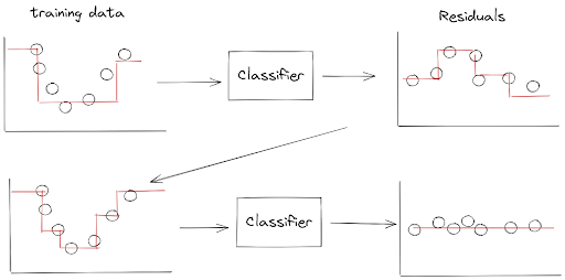
As you can see from the visualization above, we train the first classifier like normal in the first step. Then, the next classifier will be trained based on the residual errors of the previous classifier.

Once the next classifier is trained on the residual errors, we can update the ensemble model prediction by simply adding up the prediction of the next classifier with the previous classifier.

Same as AdaBoost, we can implement Gradient Boosting with the help of scikit-learn library, as you can see in the following code snippet.

from sklearn.ensemble import GradientBoostingClassifier

gb_clf = GradientBoostingClassifier(n_estimators=10)
gb_clf.fit(X_train, y_train)

Gradient Boosting can be used for data points that are not linearly separable as well. Below is the visualization of the decision boundary drawn by a Gradient Boost model on the data points presented in the previous section.

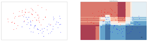
As you can see, it also achieves an accuracy of 95%, and is very much comparable with other ensemble-based classification algorithms in machine learning such as AdaBoost and Random Forest presented in the previous sections.

Conclusion

And that’s all. We have come to the end of this article! In this article, we’ve learned about various classification algorithms in machine learning and the common metrics to assess their performance. We hope that this article is useful to help you to get more familiar with classification algorithms in machine learning.