Overview of Machine Learning Algorithms: Regression

An overview of one of the most fundamental machine learning algorithms: Regression Algorithm.
Regression algorithm is one of the most fundamental machine learning algorithms out there. Doesn’t matter whether we notice it or not, we’ve come across regression problems in some stage of our life. Do you want to take a taxi to go to the airport? You got yourself a regression problem. Do you want to buy a new house? You got yourself a regression problem again.
Regression is a type of supervised learning, where we provide the algorithm with the true value of each data during the training process. After that, we can use the trained model to predict a numeric value, whether it’s a price that you should pay to buy a new house, people’s weight and height, birth rate, etc.
There are several common regression models out there, and we’re going to cover them one by one in this article. Specifically, below is the outline of what you’ll learn in this article:
- Linear regression
- Regression metrics and cost functions
- Normal equation
- Gradient descent for linear regression
- Polynomial regression
- Bias-variance trade-off
- Regularized linear model (Ridge Regression, Lasso Regression, ElasticNet)
- Support Vector Regression
- Decision Tree Regression
So without further ado, let’s start with the simplest model of them all, linear regression.
An Overview of Common Machine Learning Algorithms Used for Regression Problems
1. Linear Regression
As the name suggests, linear regression tries to capture the linear relationship between the predictor (bunch of input variables) and the variable that we want to predict. To understand this concept, let’s take a look at the common examples of regression problem:
- You want to take a taxi to go to the airport. The further the distance between your house and the airport, the more expensive the taxi fare will be. In other words, the taxi fare linearly correlates with the distance.
- You want to buy a new house. The bigger the house that you want to buy, the more you need to pay for the house. In other words, the house price linearly correlates with the house size.
Below is the equation of linear regression at the simplest form:
where:
ŷ: predicted value
θ₀: the intercept
θ₁: the weight of the first predictor
x₁: the first predictor’s value
To make the equation above more intuitive, let’s use the taxi example from above. Let’s say we want to predict how much money we need to spend for a taxi to get us to the airport. If we put this problem into linear regression equation as above, then we have:
- The taxi fare as the predicted value (ŷ)
- The distance between your house and the airport as the predictor value (x₁)
- You can imagine the intercept as the initial price that you need to pay as soon as you get in the taxi. If you notice, the taxi fare wouldn’t start at 0 whenever you get in the taxi, but at some price, let’s say $5. This $5 is the intercept (θ₀).
- You can imagine the weight of the predictor as the amount of money that you need to pay as soon as the distance traveled by the taxi increases by 1 km (θ₁).
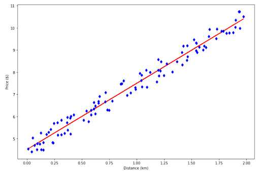
Now let’s say we have gathered the data about taxi fare with respect to the distance, and your data looks like the following.

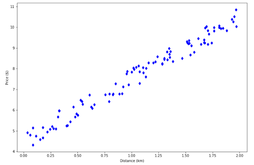
To predict the money you need to spend for a taxi, you would need a red line below:

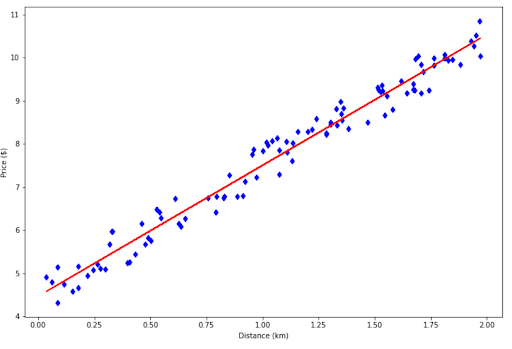
The red line above is called a regression line. Thanks to this regression line, now you can estimate the amount of money that you need to spend depending on the distance between your house and the airport.
The natural question that comes after this is: how do we get the regression line as above?
And this is where we need to know different kinds of metrics and cost functions for regression problems.
2. Regression Metrics and Cost Functions
The regression line that you see from visualization above should be the line that gives the best fit possible considering the data points that we have.
To get the line with the best fit, we should have something to measure. In a regression problem, we use metrics and cost functions to measure the goodness of the regression line to capture the pattern of our data points.
Although they might be similar, there is a distinction between metrics and cost functions.
- Metric is a value that we use to assess the performance of our regression line (i.e how good is the fitted line produced by the model to capture the pattern of our data).
- Cost function is a value that our regression model tries to minimize during training (i.e with Gradient Descent algorithm)
In terms of a regression problem, we normally use the same value for the metric and cost function, while in a classification problem, the metric and cost function can be different.
So, what are these metrics and cost functions that we normally use for a regression problem? Let’s start with Mean Squared Error.
Mean Squared Error (MSE)
Mean Squared Error (MSE) is the most common metrics used for regression analysis. It measures the goodness of fit of our regression line by measuring the sum of squares of prediction error made by our regression line as you can see from the equation below.
where:
N: total number of data points
yi: the actual value of each data point
ŷi: the value of each data point predicted by regression line
From the equation above, we can see that the bigger the difference between the actual value and predicted value, the bigger the MSE would be. Small MSE means that our regression line did a good job in predicting the value of our data points and vice versa.
There are two reasons why we need to square the difference between the actual and predicted value of each of our data points according to the equation above:
- To make sure that we have a positive error value
- To ‘punish’ the regression model when the error is large
Root Mean Squared Error (RMSE)
As the name suggests, Root Mean Squared Error (RMSE) is an extension of MSE. It’s basically just a square root of MSE, as you can see from the equation below.
You might be wondering why we should compute the square root of MSE. The reason is quite simple: just for convenience. It makes sure that the units of the error are the same as the units of the value that we want to predict.
Using the example above, let’s say that we want to predict a taxi fare and our unit is in ‘dollars’. The square root operation makes sure that our RMSE would also be in ‘dollars’, not ‘squared dollars’.
Mean Absolute Error (MAE)
Mean Absolute Error (MAE) is also one of the most common metrics for a regression problem because it has the same unit as the value that we want to predict, just like RMSE.
What differentiates MAE from the other two metrics above is how it accumulates the error. Unlike MSE and RMSE, MAE doesn’t magnify the prediction error by squaring the difference between the actual and predicted value of each data point.
As you can see from the equation above, there is not much difference between the equation of MAE and the other two metrics. It uses an abs operator to make sure that we have a positive error value.
You can use any of the three metrics mentioned above for a regression problem. However, in this article we’re going to use MSE as our regression metrics and cost function.
Now a natural question that should come up is: we know how to measure the goodness of our regression line, but how do we improve it? In other words, how can our model create a regression line that minimizes the MSE value?
To minimize the MSE value, we need to train our regression model on the available data points. There are two ways to minimize MSE value and train a regression model: using the Normal Equation and using a Gradient Descent algorithm.
We’re going to cover both methods, and let’s start with the Normal Equation.
3. Normal Equation
Normal Equation is a closed-form solution that is only available in a regression problem. With this equation, you can get a regression line with the best possible fit in a split second.
Computing the Normal Equation requires knowledge in linear algebra because it deals with matrix multiplication and matrix inversion extensively. The general equation for Normal Equation is as follows:
where:
θ̂ : the weight values of intercept and each predictor that minimizes the cost function
X: the predictor matrix
y: the vector of true values of each data point
As the number of predictors increases, the computation would be more complicated. However, we can compute this easily with Python as you can see below.
import numpy as np
import matplotlib.pyplot as plt
%matplotlib inline

# Generate data
np.random.seed(42)
x = 2 * np.random.rand(100,1)
y = 4 + 3 * x + np.random.rand(100,1)

x_b = np.c_[np.ones((100,1)), x] #for intercept

# Compute normal equation
theta_hat = np.linalg.inv(x_b.T.dot(x_b)).dot(x_b.T).dot(y)
print(theta_hat)

# Output: array([[4.51359766],
       [2.98323418]])
As you can see in the code snippet above, we get an output that has two values: one for the intercept and another for the weight of our predictor. These values are the optimum values for both parameters such that we get the regression line with the best possible fit.
Finally, we can visualize the regression line with the following code:
# Create regression line
x_new = np.array([[0], [2]])
x_new_b = np.c_[np.ones((2,1)), x_new]
y_new = x_new_b.dot(theta_hat)

# Plot regression line
plt.figure(figsize=(12, 8))
plt.plot(x_new, y_new, 'r-')
plt.plot(x,y,'bd')
plt.xlabel('Distance (km)')
plt.ylabel('Price ($)')
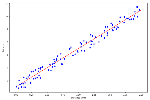
With the regression line that we see above, now we can predict the taxi fare depending on the distance. Let’s say that we know that our house is 1.5 km away from the airport, we can use this regression model to predict the taxi fare as follows:
x_new = np.array([[1.5]]) # Our distance
x_new_b = np.c_[np.ones((1,1)), x_new]
y_new = x_new_b.dot(theta_hat)

print(y_new)

# Output: array([[8.98844892]])
As you can see, the regression model predicts that we have to pay approximately $9 if we want to take a taxi to the airport.
There are two advantages of using Normal Equation to find a regression line with the best fit:
- It is very straightforward to implement
- It’s very scalable if we have a lot of data points (training data)
However, one drawback that we have with Normal Equation is that the more predictors we have, the slower the computation will be. This is because of the matrix inversion operation that will become more and more complicated as the number of predictors increases.
This drawback doesn’t appear if we use the second approach to find the best fit of our regression line, which is by using Gradient Descent.
4. Gradient Descent for Linear Regression
Gradient Descent is an optimization machine learning algorithm that has a goal to minimize a cost function, which in our case would be the MSE value.
If you want to understand how a Gradient Descent works, just imagine that you’re on the top of a mountain and you want to go downhill. The best possible way to do so quickly is by choosing the direction of the steepest slope.
And that’s what Gradient Descent does. It tries to minimize the cost function by choosing the direction of descending gradients at every iteration until it converges. If it converges, this means that we have reached the lowest possible value of our cost function.


To implement Gradient Descent, we need to implement two steps in every iteration or epoch:
1. Calculate the gradient of the cost function with respect to the weight of each predictor.
Or we can generalize the equation above for all predictors into the following equation:
where:
j: the total number of predictors
k: the total number of data points
The final equation on the right hand side of the equation above will come in handy when we try to implement Gradient Descent with Python later on.
2. Update the weight of each predictor by subtracting it with the gradient.
Learning Rate of Gradient Descent
From the image above, we can see that the Gradient Descent algorithm tries to minimize our cost function by going to the direction of descending gradients one step at a time. Now the question that we might ask is: can we adjust the size of the steps taken by the Gradient Descent algorithm in every iteration?
Yes, we can. There is a hyperparameter in this algorithm called learning rate, or η in the equation above, that we can tweak to adjust the steps of Gradient Descent in every iteration.
However, we need to understand the benefit and the drawback of this learning rate adjustment:
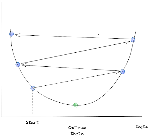
- If the learning rate is too small, then the regression model will converge very slowly and you need more training iteration for Gradient Descent to reach global minimum.
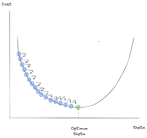
- If the learning rate is too high, then the algorithm will jump around chaotically from one side of the valley to another, which is the main cause of a divergence in our result. The cost function might grow larger than our initial value and we would never arrive at the optimum solution.

Now that we know how Gradient Descent works, let’s see different types of Gradient Descent implementation that we can use.
Batch Gradient Descent
Batch Gradient Descent is the default implementation of Gradient Descent machine learning algorithm.
It takes all of our training data into account in every iteration to minimize our cost function.
To conduct batch Gradient Descent, we need to compute the gradient of the cost function with respect to the weight of each predictor in every iteration or epoch. In other words, we want to know how much the cost function will change if we adjust the weight of each predictor a little bit.
Below is the implementation of batch Gradient Descent
# Set hyperparameters
lr = 0.01
epochs = 3000
train_data = len(x)


# For intercept
X_b = np.c_[np.ones((100,1)), x]

# Initialize weight
theta = np.random.randn(2,1)

# Gradient descent over whole data
for i in range(epochs):

      # Compute the gradient of each predictor
	grad = 2 / train_data * X_b.T.dot(X_b.dot(theta)-y)

      # Update the weight of each predictor
	theta = theta - lr*grad

print(theta)
# Output: array([[4.51354059], [2.98328456]])

# Visualize result

plt.figure(figsize=(12, 8))
plt.plot(x, theta[0][0] + x * theta[1][0], 'r-')
plt.plot(x, y,'bd')
plt.xlabel('Distance (km)')
plt.ylabel('Price ($)')
And finally we’ve got our perfectly fitted regression line!
However, as you might have guessed, one drawback of implementing batch Gradient Descent is the speed and efficiency. If you have a large set of training data, implementing batch Gradient Descent might not be the best approach as it will become slower. Hence, let’s take a look at other options.
Stochastic Gradient Descent
As the name suggests, stochastic Gradient Descent performs the minimization of cost function by randomly picking data points on our training data in every iteration. Since we’re not using the whole training data, then the training process can be much faster if we have a huge set of training data.
Below is the implementation of stochastic Gradient Descent:
epochs = 3000
lr = 0.01

theta = np.random.randn(2,1)

for i in range(epochs):

  for j in range(train_data):

    	# Choose random training data
    	idx = np.random.randint(train_data)
    	x_i = X_b[idx:idx+1]
    	y_i = y[idx:idx+1]

    	# Compute gradients based on randomly selected training data
    	grad = 2 * x_i.T.dot(x_i.dot(theta) - y_i)
    	theta = theta - lr * grad

print(theta)
# Output: array([[4.4920683 ],[2.98692425]])
If you want to have a simpler implementation than the code snippet above, then you can also utilize SGDRegressor method from scikit-learn library.
from sklearn.linear_model import SGDRegressor

sgd = SGDRegressor(max_iter=3000, eta0=0.01)
sgd.fit(x, y.ravel())

print(sgd.intercept_, sgd.coef_)
# Output: [4.1762039] [3.28159362]

# Visualize result
plt.figure(figsize=(12, 8))
plt.plot(x, sgd.predict(x), 'r-')
plt.plot(x, y,'bd')
plt.xlabel('Distance (km)')
plt.ylabel('Price ($)')

Since this machine learning algorithm picks random instances of our training data in every iteration, then you would notice that the cost function will bounce up and down at every iteration instead of continuously decreasing as you might see in batch Gradient Descent.
This would sometimes lead to a final cost function value that’s not 100% optimum, as you can see in the visualization of the regression line above.
Mini-batch Gradient Descent
The implementation of mini-batch Gradient Descent is slightly different in comparison with batch Gradient Descent and stochastic Gradient Descent, but its concept is pretty easy to understand once we know the previous two implementations.
Instead of taking the whole training data in every iteration like batch Gradient Descent or picking random instances of our training data at every instance like stochastic Gradient Descent, mini batch Gradient Descent takes the middle ground between two implementations. It splits the whole training data into several small batches and each batch consists of instances randomly sampled from our training data.
This idea allows us to get a reasonable increase in performance if we train our data with GPU. Also, the result that we get from this implementation is less ‘chaotic’ than stochastic Gradient Descent, but not as smooth as batch Gradient Descent.
However, it is important to note that training our data with mini-batch Gradient Descent is much faster in comparison with batch Gradient Descent.
If you want to learn interactively how a regression line is generated depending on our data points, check this resource.
5. Polynomial Regression
So far we’ve seen how a linear regression model produces a straight regression line that fits our data by minimizing the cost function. But can the model produce more than a straight line?
Although the model is called linear regression, it can actually produce more than just a straight line. It can also produce a curved line in case you want to fit the model on non-linear data, for example as follows:
np.random.seed(42)
x = 6 * np.random.rand(100, 1)-3
y = 2 * x**2 + np.random.randn(100,1)

plt.figure(figsize=(12, 8))
plt.plot(x, y,'bd')
plt.xlabel('x1')
plt.ylabel('y')
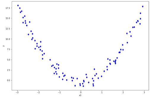
If you have data points like above, of course a regular linear regression wouldn’t cut it as it will always produce a straight line. When our fitted line is a straight line but we have non-linear data points as above, we end up with the result as follows:


As you can see, our fitted line performs poorly to represent our data points. This fitted line will perform poorly as well if we provide an unseen data point. This phenomenon is famously called underfitting, which means that our model is too simple to be able to capture the pattern of our data points.
So, what should we do to fix underfitting? We need to make a few transformations into our linear regression equation by adding higher degree predictors in the regression equation as follows.
where n is the polynomial degree that we can set in advance. After this transformation, we basically have a polynomial regression.
To transform our normal linear regression function into a polynomial regression function as above, we could use PolynomialFeatures class from scikit-learn. This class will create the powers of each predictor as additional predictors in our regression function.
from sklearn.preprocessing import PolynomialFeatures
import operator

poly_features = PolynomialFeatures(degree=2, include_bias=False)
x_poly = poly_features.fit_transform(x)
Now if you want to increase the degree of each predictor, then all you need to do is adjust the degree parameter when you initialize PolynomialFeatures instance above.
After this feature transformation, we can fit a linear regression model on this transformed feature as follows:
import operator

lin = LinearRegression()
lin.fit(x_poly, y)

# Sort value before plotting
sort_axis = operator.itemgetter(0)
sorted_zip = sorted(zip(x,lin.predict(x_poly)), key=sort_axis)
x_pred, y_pred = zip(*sorted_zip)


# Visualize the result
plt.figure(figsize=(12, 8))
plt.plot(x_pred, y_pred, 'r-')
plt.plot(x, y,'bd')
plt.xlabel('x1')
plt.ylabel('y')

And now we have a regression line that captures the pattern of our data really well!
If you want to learn more about Polynomial Regression, check out this resource.
6. The Bias-Variance Trade-Off
Now we know that we can actually fit in non-linear data with polynomial regression. The next question that might come into our mind is: what will happen if we increase the degree of each predictor further?
If we keep increasing the degree of each of our predictors, then we will get a fitting line that strictly follows each of the data points. Below is an example of this phenomenon.


This is not what we want to get from the fitted line for one obvious reason: it won’t generalize well. We would expect a poor performance if we provide an unseen data point to the model. And this is what we call overfitting.
So far, we’ve heard about two important terms that describe the performance of a regression model: underfitting and overfitting.
- Underfitting means that the model is unable to capture the pattern of training data points.
- Overfitting means that the model tries to fit each of the training data points such that it won’t generalize well on unseen data points.
If you understand these two terms, then you would understand terms like bias and variance as well.
- Bias measures the difference between mean prediction of our machine learning model with the actual value of data points that we try to predict. If our model produces a high bias, this means that our model is too simple to capture the pattern of our data. And this means we have an underfitting case.
- Variance measures the spread of model prediction for a given data point. If our model produces a high variance on an unseen data point, this means that our model is very sensitive to small changes in training data because it tries too hard to follow the pattern of our training data. And this means we have an overfitting case.
To understand bias and variance in a clearer way, below is the visualization of what it means when our model has a high/low bias and variance.


By looking at the picture above, of course, you might already know that an ideal model would be the one with a low bias and a low variance.
Controlling bias and variance can normally be done by adjusting the model's complexity (i.e whether to use a linear regression, second order polynomial regression, third order polynomial regression, and so on).
Increasing a model’s complexity would also increase its variance and reduce its bias. On the opposite side, reducing a model’s complexity would also decrease its variance, but it will increase its bias.
This is what a bias-variance trade-off is all about. What we should do is to find that sweet spot, where the bias and variance error intersect, as you can see in the image below:


From the visualization above, now we know what we should do to build our regression model that will perform well both on training data and unseen data.
- If our model produces a high bias, increase its complexity (i.e instead of linear regression, we use a polynomial regression)
- If our model produces a high variance, reduce its complexity, add more training data, or apply regularization techniques, which we will cover in the next section.
7. Regularized Linear Model
As stated above, regularization is a technique that we can implement to combat overfitting. What this technique does is that it will add an additional constraint to the weight of each predictor.
There are three types of regularized linear model that’s commonly applied in practice: Ridge Regression, Lasso Regression, and Elastic Net. Let’s start with Ridge Regression.
Ridge Regression
Ridge Regression has an additional term in its cost function in comparison with regular linear regression, as you can see in the following equation:
where:
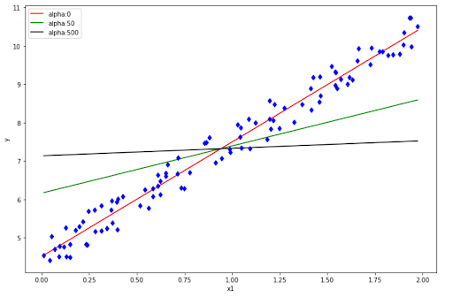
- α: a hyperparameter that controls how much you want to regularize your linear regression model.
- θi: the weight of each predictor
The main goal of this additional term is to keep the weights of our model to be small during the training process.
If you set α to be 0, then this Ridge Regression turns into a regular linear regression. Meanwhile, if we set α to a large number, then all of the weights become very close to zero. This will turn the fitted line to be no other than a flat line through the mean value of data points.

It’s very straightforward to implement Ridge Regression with scikit-learn library, as you can see below:
from sklearn.linear_model import Ridge

ridge = Ridge(alpha=1)
ridge.fit(x,y)
Lasso Regression
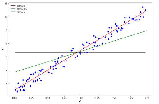
Lasso is actually an abbreviation that stands for Least Absolute and Selection Operator. The good thing is, the implementation of Lasso Regression is very similar to Ridge Regression, as you can see from the following cost function:
The additional term that we add with Lasso Regression is similar to Ridge Regression. The difference is that instead of squaring each predictor’s weight (l2 norm), we’re using the abs operator (I₁ norm) instead.
The intuition is still the same as Ridge Regression. If you set α to zero, then we end up with regular linear regression. Meanwhile, if we set α to a large number, then we end up having a flat line that goes through the mean value of our data.
To implement Lasso Regression with scikit-learn, we can do the following:
from sklearn.linear_model import Lasso

lasso = Lasso(alpha=0.1)
lasso.fit(x,y)
Check out this resource if you want to learn more about Ridge Regression and Lasso Regression!
Elastic Net
Elastic Net can be seen as the combination between a Ridge Regression and a Lasso Regression, as you can see in the cost function equation below.
From the equation above, we have one additional term called r, which is our I₁ ratio. If you set the I₁ ratio to 1, then we have a pure Lasso Regression. Meanwhile, if you set the I₁ ratio to 0, then we have a pure Ridge Regression.
Implementing Elastic Net with scikit learn is also as straightforward as the other two regularized linear models, as you can see below.
from sklearn.linear_model import ElasticNet

elastic_net = ElasticNet(alpha=1, l1_ratio=0.5)
elastic_net.fit(x, y)
8. Support Vector Machine Regression (SVM Regression)
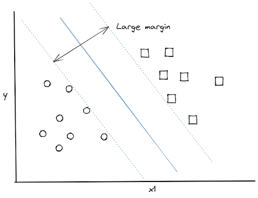
Support Vector Machine (SVM) is a machine learning algorithm that is more commonly used for classification tasks. The fundamental principle of the SVM algorithm is to create a hyperplane to separate data points with the largest margin. As an example, let’s consider the following data points:


We have many different options to draw a hyperplane that separates two data points distinctively, the optimum one would look like this:

It turns out that we can use the concept above to solve a regression problem. The difference is:
- In a classification problem, we ask the SVM algorithm to create a hyperplane with the largest possible margin to separate data points with different classes.
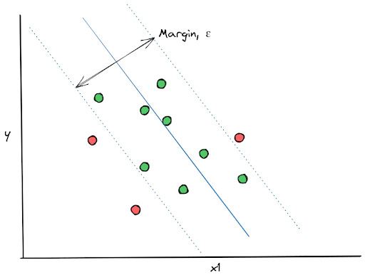
- In a regression problem, we ask the SVM algorithm to create a hyperplane with a margin that fits as many data points as possible.
The concept of SVM Regression itself is also different to the typical Gradient Descent based regression algorithm like Ridge regression, Lasso regression, and Elastic Net above.
With SVM Regression, our main goal is not to minimize the cost function, but to create a regression line with the error within a certain acceptable range. To do this, first we set the maximum error, ε, and then the SVM Regression tries to find a hyperplane (or regression line) that fits our data points while fulfilling the maximum error that we specified in advance.

To implement linear regression with SVM Regression, you can use scikit-learn library as follows:
from sklearn.svm import SVR

np.random.seed(42)
x = 2 * np.random.rand(100,1)
y = 4 + 3 * x + np.random.rand(100,1)

svr = SVR(kernel = 'linear', epsilon = 0.1)
svr.fit(x,y.ravel())

# Plot result
plt.figure(figsize=(12, 8))
plt.plot(x, svr.predict(x), 'r-')
plt.plot(x,y,'bd')
plt.xlabel('x1')
plt.ylabel('y')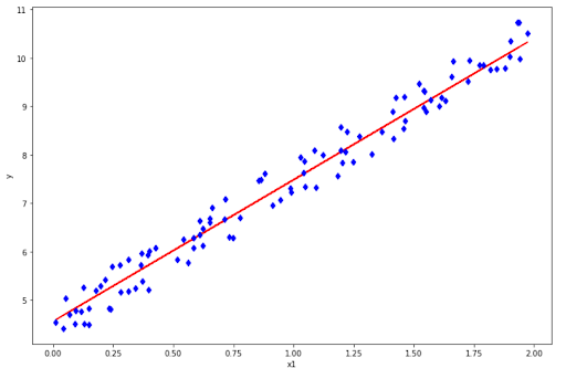
Not only for linear data points, SVM Regression can also be used for nonlinear data points. All you need to do is change the kernel of the SVM and choose the polynomial degree that you want as follows:
svr = SVR(kernel = 'poly', degree= 2)
svr.fit(x,y.ravel())
If you want to learn more about the theory behind Support Vector Regression, check out this resource.
9. Decision Tree Regression
Decision Tree is also one of the machine learning algorithms that's commonly used for classification, but it can also be used for a regression task.
A Decision Tree consists of three parts: root node, interior node, and leaf node, as you can see in the image below.

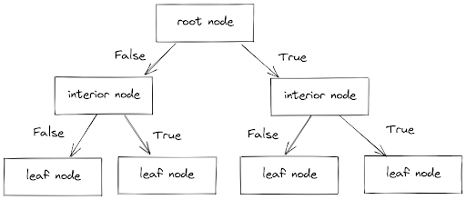
For each of our data points, it runs through from the root node until it reaches the leaf node by answering a series of True or False conditions in the interior nodes. Finally, the leaf node will give the outcome of each of our data points.
The concept between Decision Tree for classification and regression is similar. The only difference is:
- In a classification task, the Decision Tree predicts a class in each node.
- In a regression task, the Decision Tree predicts a continuous value in each node.
It’s very simple to implement Decision Tree Regression with scikit-learn, as you can see below.
from sklearn.tree import DecisionTreeRegressor

np.random.seed(42)
x = 2 * np.random.rand(100,1)
y = 4 + 3 * x + np.random.rand(100,1)

tree = DecisionTreeRegressor()
tree.fit(x, y)

# Visualize regression line
x_grid = np.arange(min(x), max(x), 0.01)
x_grid = x_grid.reshape((len(x_grid), 1))
plt.figure(figsize=(12, 8))
plt.plot(x_grid, tree.predict(x_grid), 'r-')
plt.plot(x,y,'bd')
plt.xlabel('x1')
plt.ylabel('y')
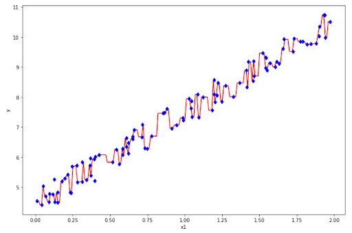
However, the result above is not what we want, since it overfits the data. This is the common problem with Decision Tree Regression, it’s prone to overfitting.
This overfitting commonly occurs when we set all of the hyperparameters to the default value (i.e we do not specify the maximum depth of the tree). To avoid this, we can play around with max_depth parameter when we initialize the model with scikit-learn.
from sklearn.tree import DecisionTreeRegressor

tree = DecisionTreeRegressor(max_depth=3)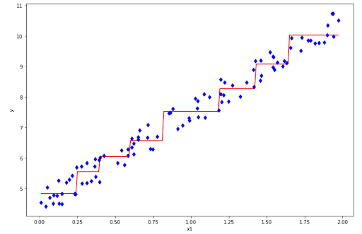
And it looks better than our previous model! One main idea to combat an overfitting problem in Decision Tree Regression is to create an additional constraint when you build the model, i.e by limiting the depth of the tree or limiting the number of leaf nodes.
If you want to see the visualization behind this Decision Tree Regression algorithm, check out this resource.
Conclusion
In this article, we have discussed an overview about common machine learning algorithms used for regression problems: such as linear regression, Ridge Regression, Lasso Regression, Elastic Net, SVM Regression, and Decision Tree Regression.
The main goal of those machine learning algorithms is to create a regression line that minimizes our cost function or metrics, such as MSE, RMSE, or MAE.
Are you ready to create your own regression project? The following resources might help you:
- If you want to get started with your own project about regression, you can check this resource to give you inspiration on where to get your dataset.
- If you want to learn how to use Python to perform a linear regression, you can check this resource or this resource.
We have also discussed the most common use case "Classification algorithm" that will also be found when dealing with machine learning. Check it here → Overview of Machine Learning Algorithms: Classification.
Latest Posts:


Share