Machine Learning Algorithms You Should Know for Data Science

Difference between Supervised and Unsupervised Machine Learning algorithms:

Supervised and unsupervised machine learning algorithms, both have different applications and both have their own strengths and weaknesses. The most common difference between these two algorithms is the way they are trained. Supervised machine learning algorithms are trained by using a labeled data set or a ground-truth label while the unsupervised machine learning algorithms are trained without the labeled dataset. Some key differences between Supervised and Unsupervised machine learning algorithms are given below:

1. Prediction vs. Insights

The end goal of a supervised learning algorithm is to predict something. For example, you will be able to train the supervised ML model which has a historically labeled dataset and use that to predict the value of a target variable. For example, if you want to predict the house price based on the number of bedrooms, area, locality, etc. you would need to train the supervised learning model to predict the house price. The unsupervised learning model does not have a target variable but it is generally used to get insights from the data. The end goal in the unsupervised learning model is to derive some insights or patterns from the data.

2. Less vs. More training data

Supervised learning models can be used even if you have a small amount of training data and it still can achieve “good-enough” results that can be used. But this is not the case with unsupervised machine learning models. These models are generally computationally expensive and need more data to find out patterns and insights from the data to get a meaningful result out of it.

3. Less vs. More time consuming

Using supervised machine learning models can be time consuming when it comes to data preparation. You would need to label the dataset beforehand, and it might take up an enormous amount of time if you have a huge dataset. Moreover, you would need domain expertise in order to accurately label each of the data points. However, for the unsupervised machine learning models you don’t need to spend a lot of time to train the model as there is no need to provide labels to each data point but the result might be highly inaccurate and it would need human decision to assess the quality and performance of the model.

Thus, if your end goal is to build a model to predict a specific outcome, then a supervised learning approach would be appropriate since it will give you a quantifiable metric that can be tracked in terms of performance. If you have a large dataset and want to gain insights into your data, then an unsupervised learning approach would be more appropriate.

There is also a middle ground between supervised vs unsupervised learning models. This approach is called a semi-supervised learning model.

Semi-Supervised Learning

A technique that fills the void between the supervised learning approach and the unsupervised learning approach is semi-supervised learning. This method, which we might refer to as a "middle ground" approach, can reduce the negative effects of both supervised and unsupervised learning, but it won't be as effective as both methods in terms of their strengths.

However, this method is quite helpful because, as you are already aware, labeling data is a time-consuming operation, and, regrettably, the majority of real-world data is unlabeled. The semi-supervised system can handle partially labeled data, which is good news.

Typically, a semi-supervised model combines an unsupervised learning model with a supervised learning model. A combination of logistic regression (supervised learning) and the k-means clustering technique (unsupervised learning), for instance, can constitute a semi-supervised model. To learn from partially labeled data, we can alternatively convert a supervised learning classifier into a semi-supervised learning classifier.

Types of Machine Learning Algorithms you should know as a Data Scientist

In this section we will discuss some of the machine learning algorithms that you should know as a Data Scientist. If you are someone who is preparing for your next Data Science interview or someone who is a seasoned Data Scientist, this section will give you a quick overview of some of the most important machine learning techniques that you should be familiar with.

1. Linear Regression

Regression is a form of supervised learning in which we train the algorithm using the real value of each piece of input. The trained model can then be used to forecast a numeric value, such as the cost of a new home, a person's weight and height, a country's birth rate, etc.

As the name indicates linear regression captures the linear relationship between the predictor (input variables also called as independent variables) and the variable to be predicted (output variable, target variable or also called as dependent variable). Let’s take a few examples in which we would need to use a linear regression:

You want to take a taxi from your house to the airport. At a very basic level, the price of the taxi would depend on how far your house is from the airport. The more the distance between your house and the airport, the higher would be the expense and inverse is also true; the lesser the distance between your house and the airport, lower would be the expense of taxi. At its simplest form, distance is one of the variables that impacts how much you would pay for the taxi. In other works, taxi fare linearly correlates with the distance.
You want to buy a house. The bigger the house that you want to buy, the more you would need to pay for the house. In simple words, the house price is linearly proportional with the size of the house.

The basic form of linear regression is as below:

\hat{y} = θ_0\ +\ θ_1x_1

where:

ŷ: predicted value
θ₀: the intercept
θ₁: the weight of the first predictor
x₁: the first predictor’s value

Now let’s take an example to understand the above equation more clearly. Let’s take an example to predict the price of bus ticket based on the distance you travel via bus. Now, to understand how much the ticket price is, we can use the equation that we discussed above:

We need to predict the bus ticket fare, and thus, it becomes our target variable (ŷ)
The bus ticket fare depends on the distance between your pick up location and the destination, and thus, distance becomes your predictor variable (x)
The intercept can be the initial price that you need to pay as soon as you get in the bus. For example, the fares wouldn’t usually start with 0 but there is a lower bound for the fare. Even if you travel for a very short distance, your bus fare would not drop below a certain threshold. For simplicity, let’s take that value as $2. So this is our intercept (θ₀)
Now you can imagine the weight of the predictor to be the amount of money that you need to pay extra as soon as the distance increases by 1km (θ₁)

Now let’s say we have captured the bus fare and the distance traveled, and it looks something like below:

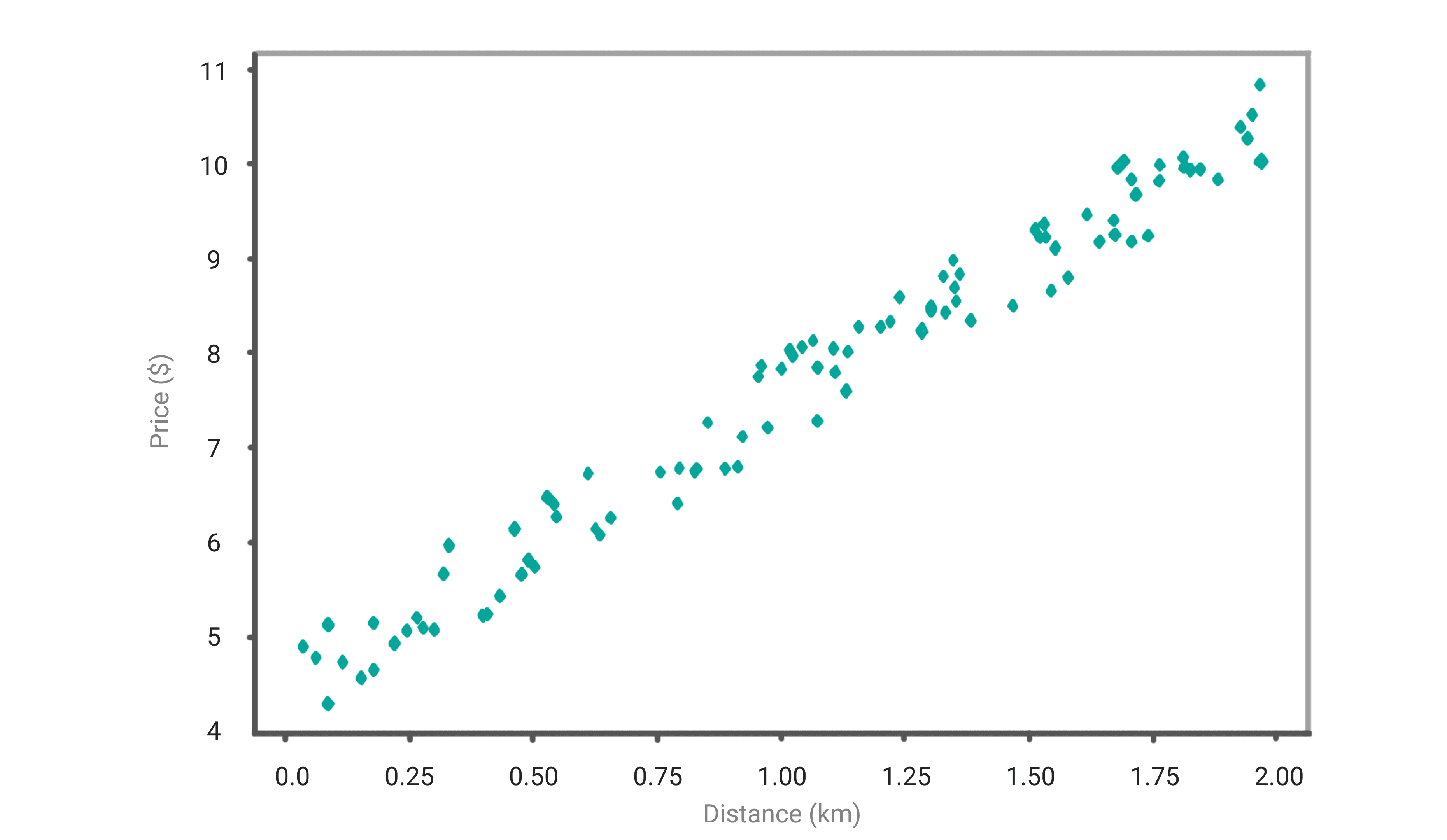
Linear Regression Machine Learning Algorithms

To predict the amount of money you would need to spend, you will need to fit a line based on the historical data. In the below graph, you can see the red line plotted.

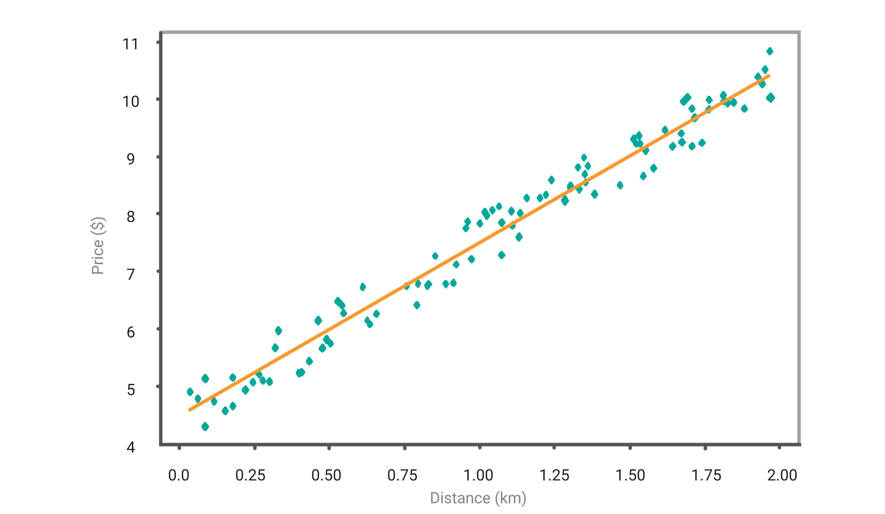
Linear Regression Example in Machine Learning Algorithms

The red line above is called the regression line, and with this, you will be able to predict the bus fare based on the distance traveled in KM. This line is also called the line of best fit. The coefficients such as (θ₀) and (θ₁) are derived by minimizing the sum of the squared difference of distance between the data points and the regression line.

The equation discussed above is an example of a simple linear regression model. Simple linear regression model has only one independent variable to predict the target variable. In our example, we used only one variable –distance– to predict the bus fare, which is our target variable. In real-world scenarios, the prediction model is not that simple. There are multiple independent variables to predict a target variable. For example, distance is one variable to predict taxi fare. Other variables could be time of the day, location, etc.

To summarize, the Linear regression model is a supervised learning model in which the model needs to be trained on the labeled data and there should be a linear relationship between independent variables and the dependent variables.

2. Logistic Regression

Logistic regression employs a similar concept to linear regression in that it uses a linear combination of the features to compute the cost function and optimize the weight. However, the name "regression" does not refer to the logistic regression process itself. Since linear regression, a machine learning approach for continuous data, is what most people envision when they think of regression, the term "logistic regression" is misleading. But logistic regression is a classification technique, not a predictor of constant variables.

The most well-known method is probably linear regression. By definition, linear regression is used when there is a linear connection between a continuous dependent variable and a continuous or discrete independent variable.

When the value of the dependent variable Y is categorical; for example, Yes or No, True or False, the subject did or did not do something, then you would need to use logistic regression. Logistic regression is used when the dependent variable is categorical and it depends on the independent variable. Linear regression usually answers the question about “How much?”. For example, how much would it cost for a taxi as in our previous example. But if we want to predict whether a taxi driver will accept your booking based on the time of day or your location, then the prediction becomes ‘Yes’ or ‘No’ as we are trying to predict whether the taxi driver will accept the booking. Such questions where the dependent variable is categorical, we can use logistic regression. Thus, logistic regression is a binary classifier, since there are only two outcomes associated with it.

In Linear regression, the trendline is a straight line and thus, it’s called linear regression. However, using linear regression, you can’t divide the output into two distinct categories- yes or no. To divide the results into two categories we need to use a sigmoid function which would clip the line between 0 and 1.

In its simplest form, the equation of the logistic regression is below:

f(x) = \frac{1}{1+e^{-x}}

Logistic Regression Machine Learning Algorithms

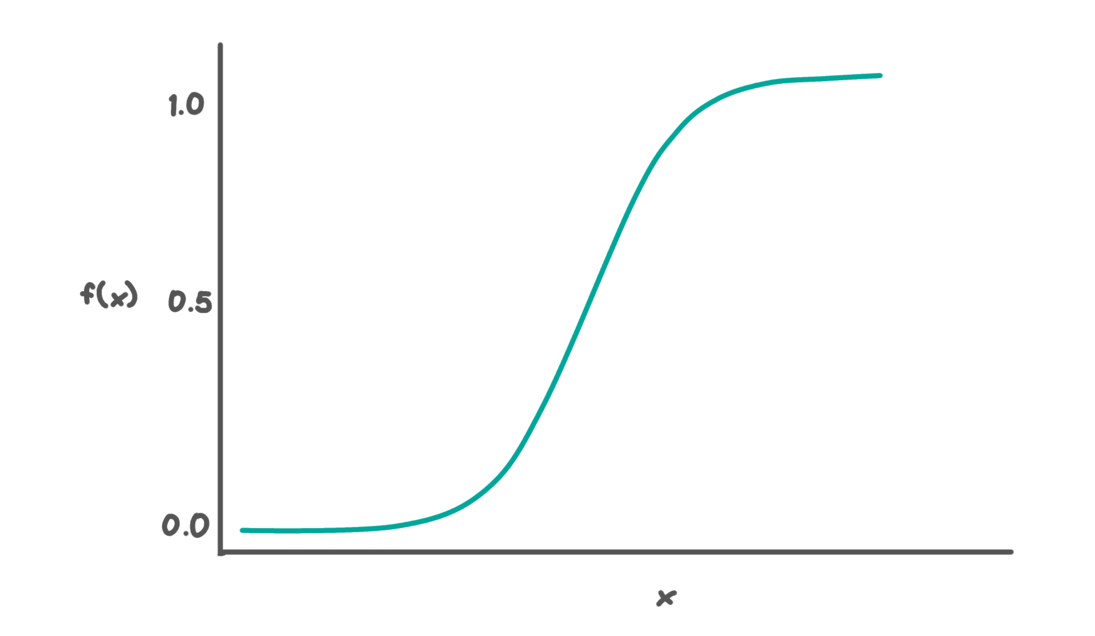
The above function is used in the Logistic Regression. This algorithm is generally used when we have a binary classification problem (a problem that has only two outcomes). Thus, we make predictions based on the value that comes from the sigmoid function above, i.e., if the value is more than 0.5, then we classify the data point as 1, and if it’s below 0.5, then we classify it as 0.

y = \begin{cases} 0,\qquad\textrm{if}\ p\ <\ 0.5\\ 1,\qquad\textrm{if}\ p\ > \ 0.5\end{cases}

To summarize, the logistic regression model should be used when the output or dependent variable is not continuous but binary. For more details on the training process for the logistic regression model, you can go through this article about classification in machine learning.

3. Decision Tree

The decision tree algorithm is one of the most popular machine learning algorithms which is a supervised learning that is used for classification tasks. The best way to comprehend a discussion of decision trees is by an analogy from daily life. Consider how frequently we are presented with situations where we must make decisions based on certain circumstances, where one decision results in a particular outcome or consequence.

Decision trees are fundamentally diagrammatic methods for solving issues. Consider the situation where, while navigating a vehicle, you must choose between making a left or a right turn at an intersection. This choice will be based on your destination.

The same logical step-by-step process is followed to get to the end stage in other situations, such as arranging a closet or purchasing a car. When purchasing a car, we research various makes and models before settling on one based on a variety of factors, including price, performance, mileage, fuel type, looks, etc.

These illustrations can serve as our use cases. Applying logic is what we must do in order to simplify a complicated situation or a complex data set. Decision trees use the same method of logical decision-making.

Approach:

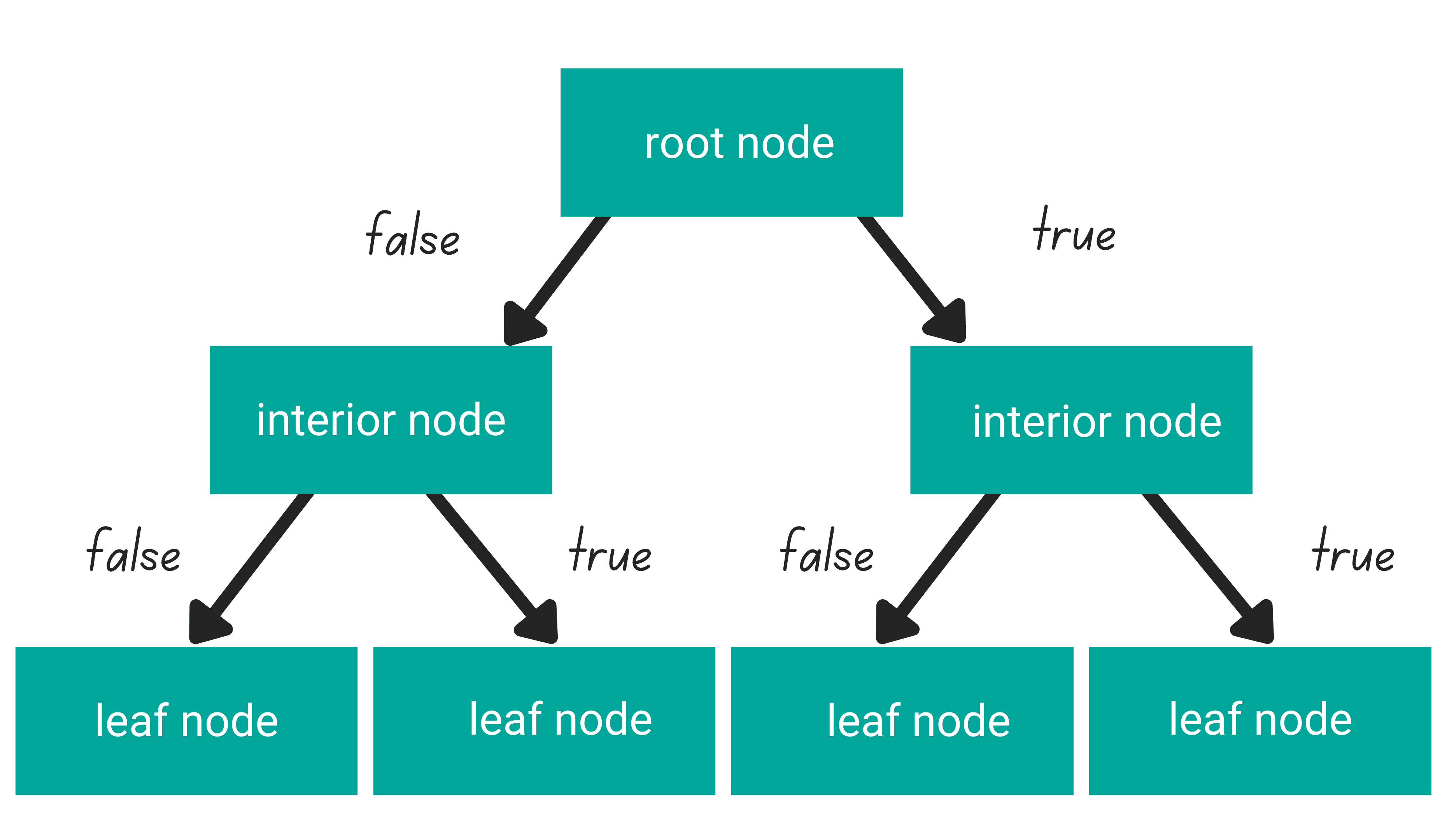
The concept of decision making based on conditions can be analyzed and shown graphically if given a problem to solve; the diagram will resemble an upside-down tree with the root at the top and branches extending downwards.

What causes this? The root represents the starting point, where we have a collection of information or choices, which we examine using a few different criteria before deciding what to do. In an inverted tree diagram, the root is known as the root node and the branches—known as the leaf nodes—represent the results of a decision.

The chance of a repeat occurrence of an attribute must be taken into account by the algorithm when finishing this segregation (considering that the same characteristic may appear more than once). As a result, the decision tree can also be referred to as a particular kind of probability tree. The amount of unpredictability or messiness in the data at the root node is known as entropy. As we divide and organize the data, we reach a greater level of precisely organized data and reach various levels of information, or "Information gain."

The Decision tree consists of a root node, a bunch of interior nodes and leaf nodes. At each level of the interior nodes, all the data points need to fulfill either a True or False condition.

Decision Tree Machine Learning Algorithm

The distinction between the Decision Tree for classification and regression is the value that we’re going to get in each of the leaf nodes. As you might have predicted, the value of the leaf nodes is continuous in regression problems and discrete in classification tasks.

4. Support-Vector Machine (SVM) Algorithm

SVM - Support-vector machines is a machine learning algorithm that is commonly used for classification tasks, although it can be used for regression problems as well. It computes the hyperplane in between two margin lines. The aim of an SVM algorithm is to build a hyperplane that divides the data in such a way that it has the highest margin between the two margin lines. Wider the margin, better separation between the two classes and thus, better performance of the algorithm.

The raw data will be plotted in an n-dimensional space where n is the number of features you have with the SVM algorithm. This data is then classified into various cohorts and plotted on a graph using lines which are known as classifiers.

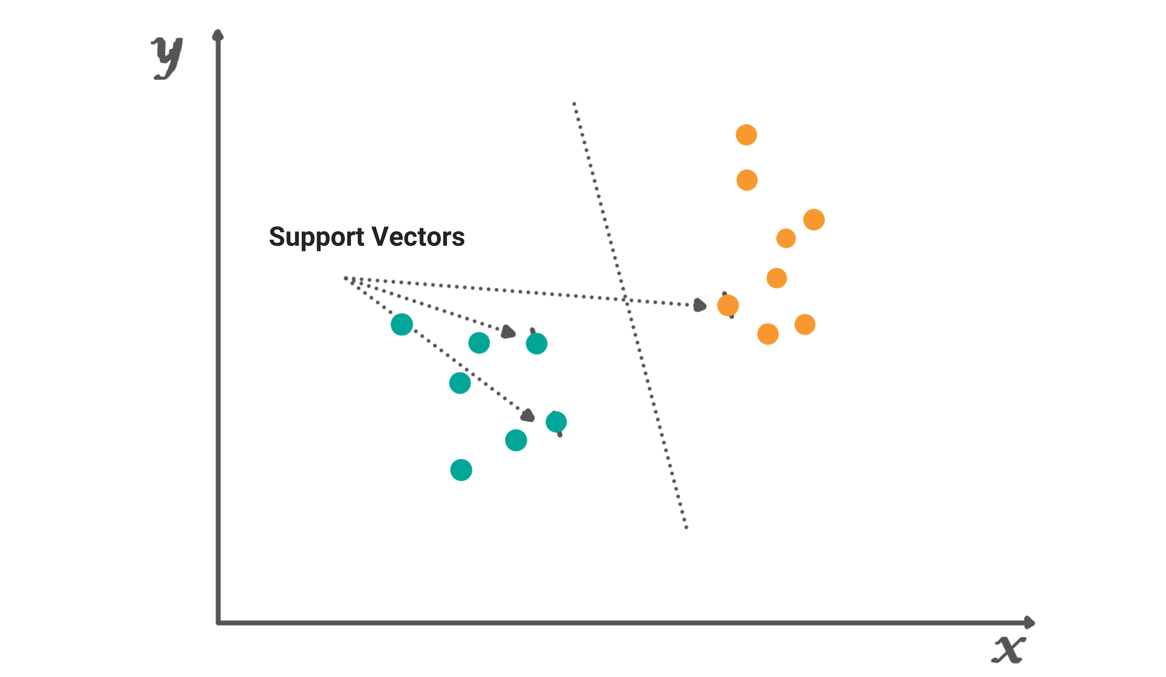
Support Vector Machine Learning Algorithm

In SVM, the model builds a line that separates the points on either side in such a way that all the points on one side of the line are as close to each other as possible while they are as far as possible to the points on the other side of the line. In the above figure, the model has built a line which separates the two classes. There can be infinite lines that separate the red and the green dots in the example above.

Support Vectors

Support vectors are the data points that are closest to the hyperplane. These are the points in the dataset that, if removed, can alter the position of the dividing hyperplane. Thus, these points are considered to be critical elements of the dataset.

Hyperplane

You can visualize a hyperplane as a line that linearly separates and categorizes a set of data for a classification problem with only two features (like the figure above).

It makes sense that the farther away from the hyperplane our data points are, the more certain we are that their classification is accurate. So, while still being on the right side of the hyperplane, we want our data points to be as far away from it as feasible.

Therefore, the class that we give to fresh testing data will depend on which side of the hyperplane it lands on.

5. Naive Bayes Algorithm

The naive Bayes algorithm is a probabilistic machine learning algorithm that is based on Bayes Theorem. This algorithm is used in a variety of classification tasks. Naive Bayes is a fantastic illustration of how the most straightforward answers are frequently the most effective. Despite recent developments in machine learning, it has shown to be not only quick, accurate, and dependable but also simple.

It has been used successfully for many things, but it excels at solving natural language processing (NLP) issues.

The Bayes Theorem is the foundation of the probabilistic machine learning method known as Naive Bayes, which is utilized for a variety of classification problems. In order to eliminate any potential for misunderstanding, we will thoroughly explain the Naive Bayes method in this post.

Bayes Theorem

Bayes Theorem is used to calculate the conditional probabilities. Conditional probability is a measure of the probability of an event occurring given that another event has already occurred. This is also called posterior probability.

P(A|B) =\frac{P(B|A)\ *\ P(A)}{P(B)}

where:

P(A|B): probability of A occurring given evidence B has already occurred
P(B|A): probability of B occurring given evidence A has already occurred
P(A): probability of A occurring
P(B): probability of B occurring

Naive Bayes has a fundamental assumption. The assumption is that each feature makes an independent and equal contribution to the outcome. For example, if you are predicting the house price based on three variables: Number of Bedrooms, Size in Sq. meters and location. The Naive Bayes theorem run unders the assumption that:

No pair of features are dependent. For example, the Size of the house has nothing to do with the other features such as the number of bedrooms and the location of the house. Thus, it considers all the features to be independent.
Secondly, each feature has equal weightage or influence on the dependent variable. For example, knowing only the number of bedrooms and size of the house won’t help us in predicting the house price. Thus, it assumes that all the features have equal weightage.

These assumptions made by Naive Bayes are generally not correct in the real-world situations. The independence assumption is almost never correct but it works well in practice and thus, the name ‘Naive’.

How Naive Bayes Algorithm works:

Let’s understand it through an example. Below we have created an example data which tells you when the F1 race completed successfully and what the temperature was like. Here the goal variable is the race status while the predictor variable is the temperature.

Dataset:

Temparature in Celcius	Race Status
negative	No
negative	No
negative	No
negative	Yes
Greater than 35	Yes
Greater than 35	Yes
Greater than 35	Yes
Greater than 35	Yes
Greater than 35	No
Greater than 35	Yes
20 to 35	Yes
20 to 35	No
20 to 35	No
20 to 35	Yes
10 to 20	Yes
10 to 20	Yes
10 to 20	Yes
0 to 10	Yes
0 to 10	No
0 to 10	No
0 to 10	Yes

Step 1: Convert the data into a frequency table. This helps us in categorizing whether the race will commence or not depending on the temperature. We have converted the above dataset into a frequency table.

Temperature in Celcius	Yes	No
negative	1	3
Greater than 35	5	1
20 to 35	2	2
10 to 20	3	0
0 to 10	2	2
All	13	8

Step 2: Create a likelihood table by finding the probabilities. From the below table, the probability of greater than 35 temperature is 0.28 while the probability of the race commencing is 0.61.

Temperature in Celcius	Yes	No	Probability (fraction)	Probability (decimal)
negative	1	3	4/21	0.1904761905
Greater than 35	5	1	6/21	0.2857142857
20 to 35	2	2	4/21	0.1904761905
10 to 20	3	0	3/21	0.1428571429
0 to 10	2	2	4/21	0.1904761905
All	13	8
	13/21	8/21
	0.619047619	0.380952381

Step 3: Calculate the posterior probability for each class using the Naive Bayes equation. The class with the highest probability is the outcome of prediction.

Hypothesis: “Race will commence if the temperature is more than 35?”. Is this correct?

We can solve this by using the posterior probability method:

\begin{aligned} P(Yes|\ Greater\ than\ 35) &= \frac{P(Greater\ than\ 35|\ Yes)\ *\ P(Yes)}{P(Greater\ than\ 35)} \\ \\ & = \frac{\frac{5}{13}\ *\ \frac{13}{21}} {\frac{6}{21}} \\ \\ & = \frac{0.38*0.62}{0.28} \\ \\ & = 0.84 \end{aligned}

Thus, we can say that the probability that the race will commence given the temperature is more than 35 is 0.84, which is high. A similar approach is used by Naive Bayes to forecast the probability of various classes based on various attributes. This algorithm is mostly used in text classification and with problems having multiple classes.

6. K - Nearest Neighbors (KNN) Algorithm

The supervised learning technique K-nearest neighbors (KNN) is used for both regression and classification. By calculating the distance between the test data and all of the training points, KNN tries to predict the proper class for the test data. Then choose the K spots that are closest to the test data. The KNN method determines which classes of the "K" training data the test data will belong to, and the class with the highest probability is chosen. The value in a regression situation is the average of the 'K' chosen training points.

For example, in the below graph, imagine there are two categories; category A which is in blue color and category B which is in red color. Now, we have a new data point in green as in the given figure and the question is to decide which category this new data point belongs to.

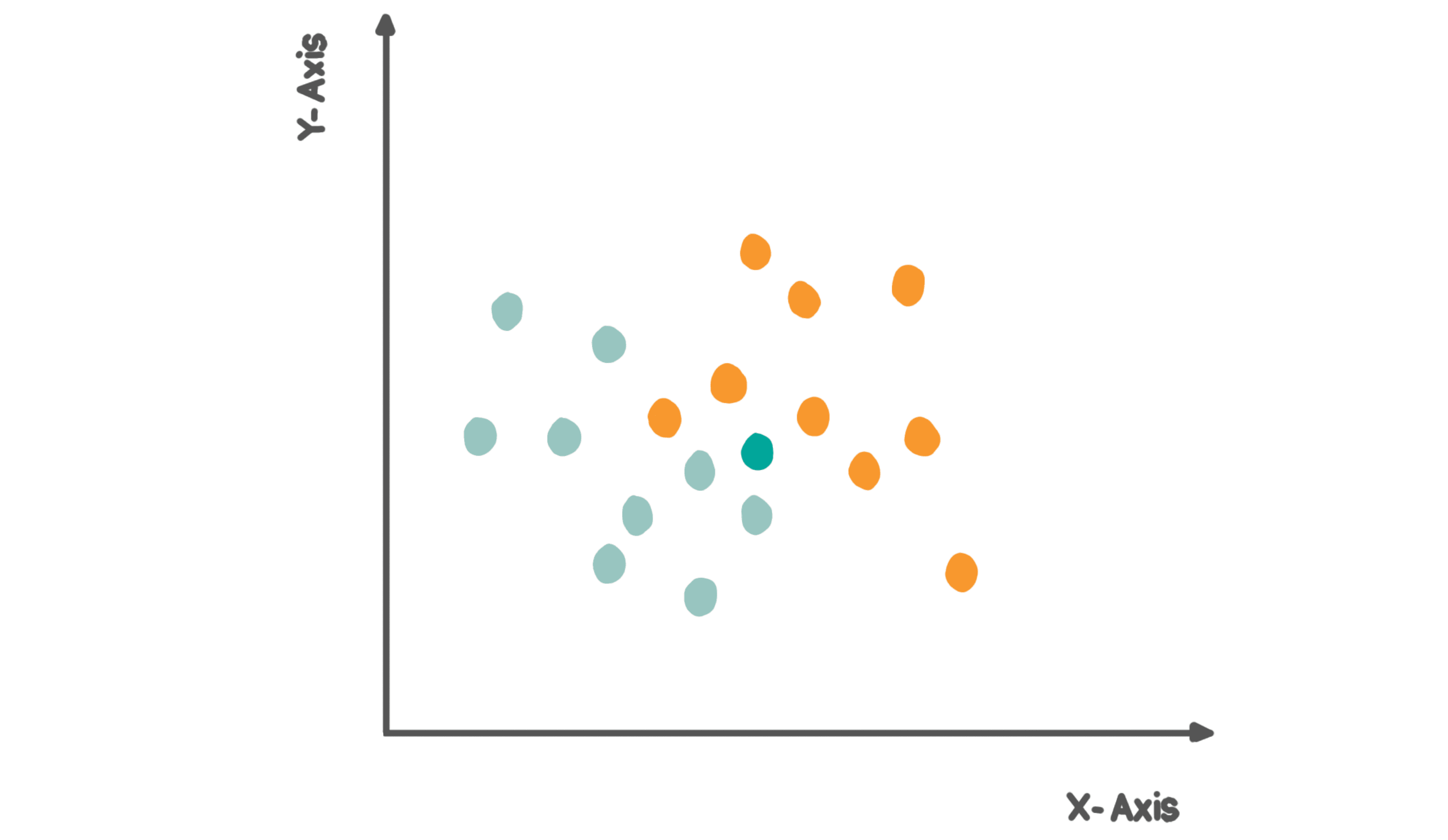
K Nearest Neighbors Machine Learning Algorithm

In the above figure, we have a total of 9 data points in the blue category and 9 data points in the red category. To classify the new point into either a red or blue class, it uses the principle of calculating distances between its neighbors. Below are the steps:

Select the value of K. K is the number of nearest neighbors.
Calculate the Euclidean distance between the new data point and its K number of neighbors. If the value of K is 4, then the new data point will calculate the distance with all the 4 nearest neighbors and check which category they belong to.
Take the K nearest neighbor as per the distance calculated
Out of these k neighbors, count the number of data points in each category
Assign the new data point to that category for which the number of neighbors is maximum

K value indicated the count of the nearest neighbors. We need to calculate the distances between the test points and the trained labels points. KNN falls under a lazy learning algorithm because updating the distance metrics with every iteration is computational.

Finding the value of K becomes critical. There is no pre-defined statistical method to find the most favorable value of K. Start with a random value of K and start computing.

In order to choose the value of K, don’t start with too small a value since it leads to unstable decision boundaries. Ideally the decision boundaries need to be smooth and for that a substantial value of K is required.

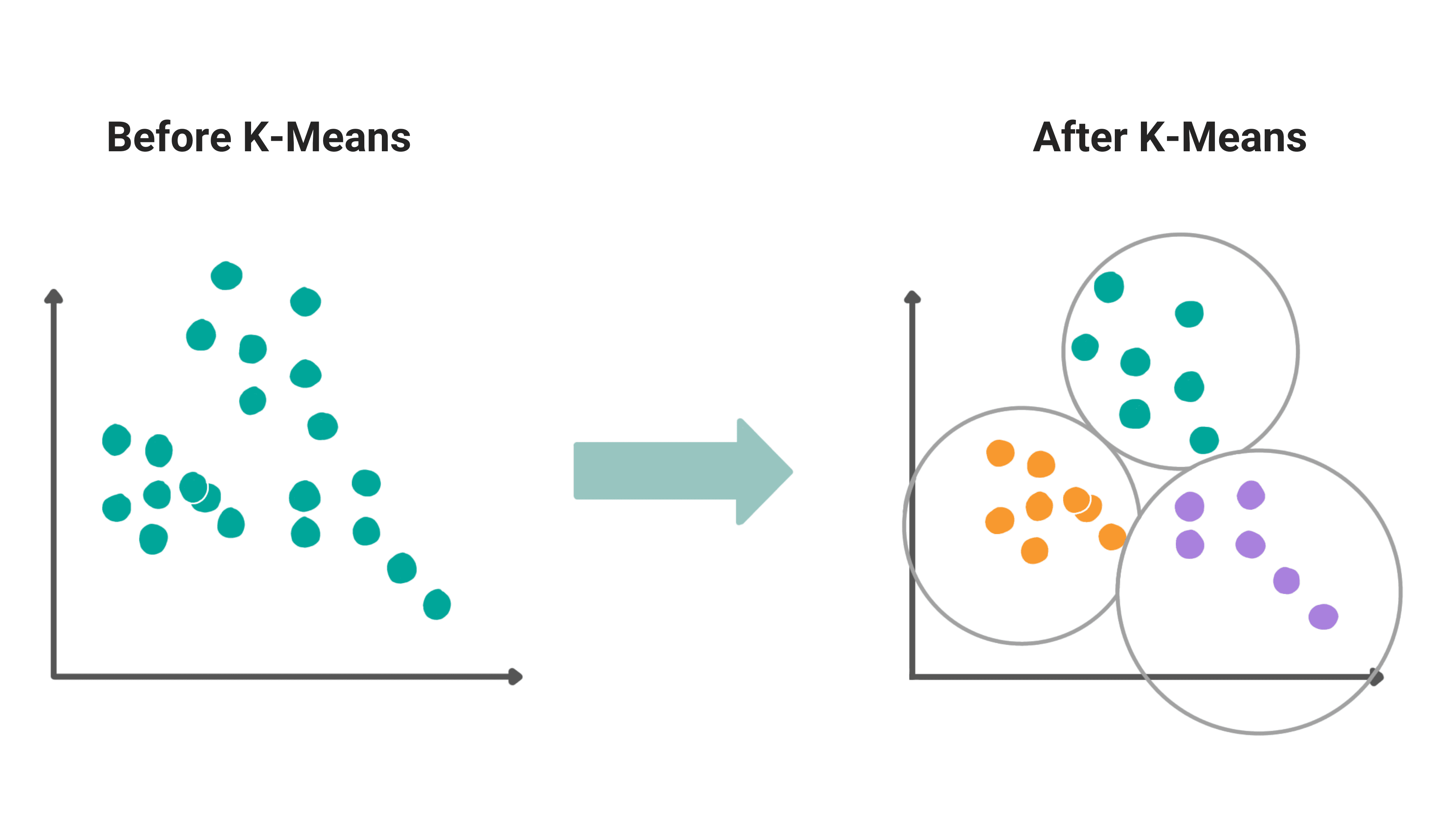
7. K - means

K- means algorithm falls under the unsupervised algorithm category. This algorithm is used to solve the clustering problems in machine learning which groups the unlabeled dataset into different clusters.

K in K-means is for the number of clusters. If the value of K = 2, then the dataset will be divided into 2 clusters, if the value of K = 4, then the dataset is divided into 4 clusters and so on. This is an iterative algorithm which divides the data into k clusters in such a way that each dataset belongs only to one group and has very similar properties.

This is a centroid-based algorithm, meaning, each cluster will have a centroid associated with it. The main goal of the algorithm is to minimize the sum of distances between the points that belong to the same cluster while maximizing the distance between the data points that belong to different clusters. As we mentioned earlier, this is an iterative process and thus, the data will be divided into k-number of clusters nad the process will be repeated until it does not find the best clusters. There are two major steps in this algorithm:

Find the best value of K centroids by an iterative process
Assign each data point to its closest cluster. Data points which are close to the particular centroid, create a cluster.

Step-by-step algorithm:

Step 1: Select the number K to decide the number of clusters
Step 2: Randonmly select the K points or centroids. This can be either an inout from the user or you can programmatically select at random.
Step 3: Once the centroids are selected in step 2, assign each data point to the nearest centroid which will form the initial clusters
Step 4: Calculate the variance and place a new centroid of each cluster
Step 5: Once the new centroids are calculated, repeat step 3 where each data point will be resigned to the new centroid and thus, a new cluster
Step 6: If there is any reassignment, then go to step 4 and if the clusters don’t change then the model is ready.

If you want details about this algorithm, you can refer to this resource.

8. Random Forest Algorithm

Similar to the KNN algorithm that we discussed earlier, random forest can also be used for both classification as well as regression problems in Machine Learning. It belongs to the supervised learning technique and thus needs labeled data for training purposes.

This algorithm is based on something called ensemble learning. Ensemble learning is the way in which an algorithm is dependent on the combination of multiple classifiers to solve complex problems and to improve the performance of the model. In the random forest algorithms, these multiple classifiers are usually the number of decision trees built on various subsets of the given dataset and then taken as an average to improve the prediction accuracy of the dataset.

Thus, instead of relying on the predictions from just one decision tree, a random forest model takes predictions from multiple trees and based on the majority votes of the predictions, it predicts the final output. More the number of trees in the random forest, higher is the accuracy and can help in preventing the overfitting problem.

Random forest works on two techniques; Bagging and Boosting.

Bagging creates a different training subset from sample training data with replacement and the final output is based on majority voting. This can be observed in the above screenshot.

Boosting combines weak learners into strong learners by creating sequential models that the final model has the highest accuracy. Random forest falls under bagging while algorithms such as ADA BOOST, XGBOOST falls under boosting.

Step by step algorithm:

Random Forest Machine Learning Algorithm

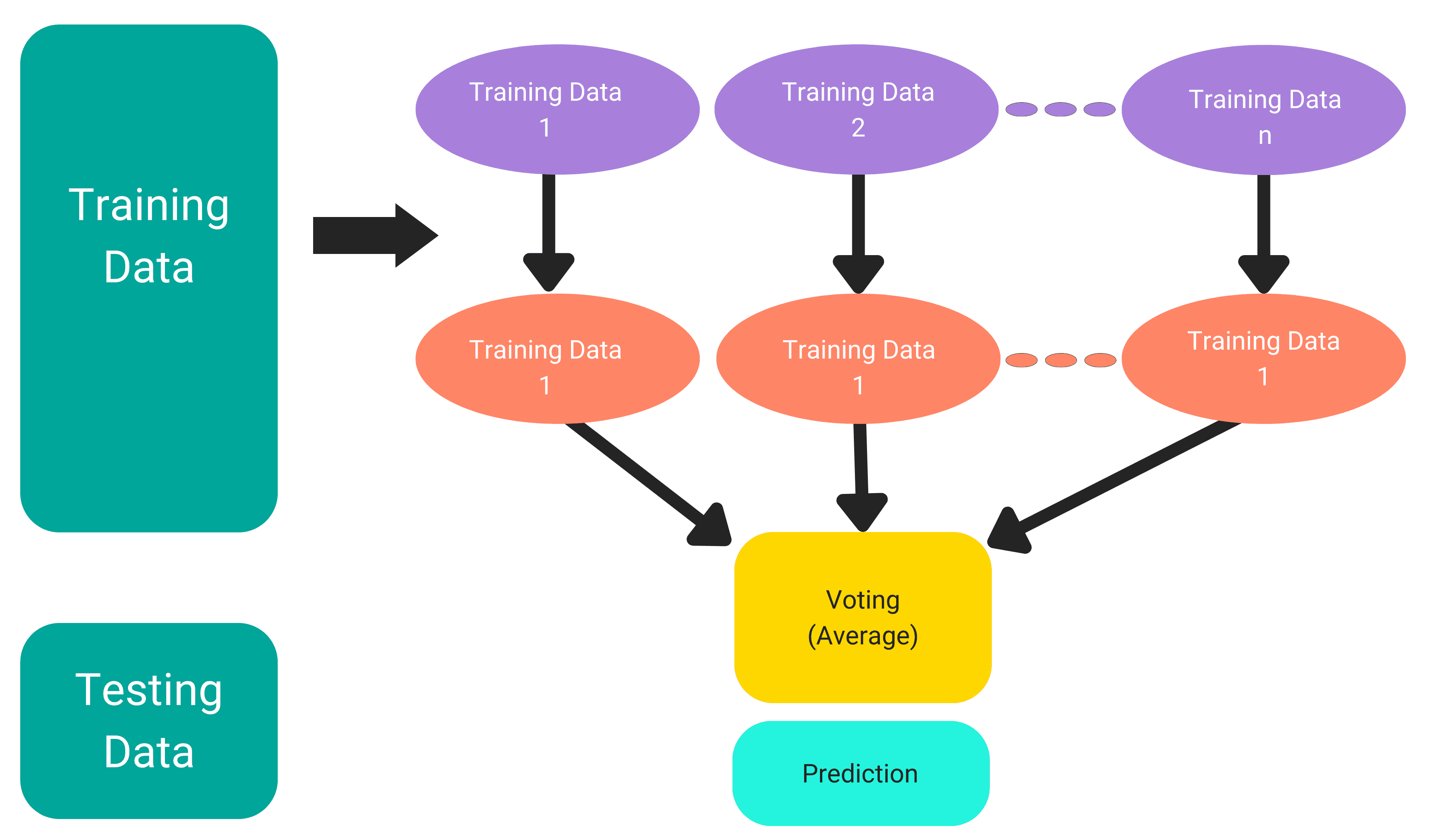
The above diagram shows the basic working of Random Forest Model. It usually works in two phases; the first step is to create the random forest by combining N decision trees and the second step is to make predictions for each tree created in the first phase.

From the Training dataset, select K random data points
Implement decision tree algorithm to these subsets of data
Choose the number of decision trees that you want to build which is denoted by N
Repeat Step 1 and 2
When the new data point comes in, predict the category for that data point by using the decision trees built on the subset and the based on the majority votes, the new data point will be classified.

As an example, please refer to the diagram below:

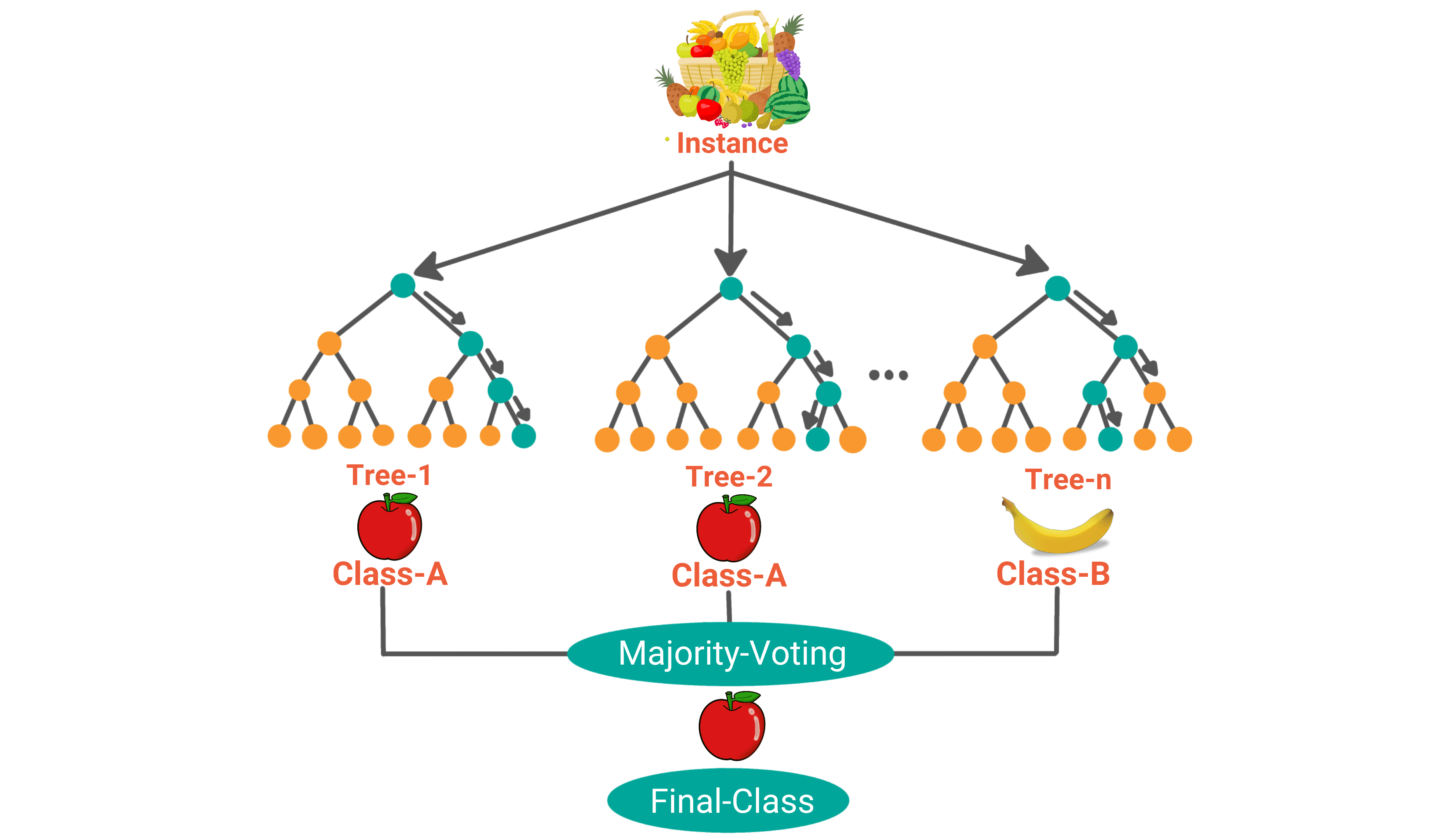
Diagram example of random forest machine learning algorithm

Now let's imagine a scenario where you have a data set of fruit images and there are multiple fruits in the data. The dataset is fed to the random forest classifier.

As the first step, the random forest classifier would build decision trees based on the subset of data.

When a new data point comes in, all the decision trees in the random forest model will classify the new data point into a relevant category. For example, from the above image, we see the first tree has classified the image as an apple, the second tree has classified the new image as an apple and the nth decision tree has classified the new image as a banana.

The last step is voting. It finds which class has gotten the maximum votes and based on that, the random forest classifier classifies the data.

Conclusion

In this article, we introduced the concepts of supervised learning algorithms, unsupervised learning algorithms and semi supervised learning algorithms. Data Science interviews can be overwhelming with such a wide syllabus to study. In this article we looked at 8 must-know machine learning algorithms if you are interviewing for your next data science job.

We also looked at the difference between Supervised vs. Unsupervised algorithms. This is one of the most common interview questions. If you are interested in expanding your knowledge in machine learning, StrataSratch has great resources.