In this article, we’ll discuss advanced SQL concepts and their use cases. Then we’ll use them to answer interview questions from reputable employers.

SQL is an essential skill for working with databases. It allows beginner data scientists to easily select, filter, and aggregate data. You can even combine some of these basic SQL features to perform more difficult tasks.

SQL also has more advanced features, which allow you to perform difficult tasks using fewer lines of code. In this article, we’ll discuss useful but lesser-known advanced SQL features for writing more efficient queries.

We will also discuss advanced use cases for familiar SQL features. For example, how to use GROUP BY statements to calculate subtotals.

Concepts to Write Advanced SQL Queries

Let’s take a look at some of the most useful advanced SQL concepts and their use cases.

JOINs

JOINs are among the essential SQL features, often used to combine tables based on relationships between them. Normally, JOINs do not increase the volume of records, only the breadth of information.

In practice, you will often encounter cases when necessary information is stored in two different tables. You can use JOINs to ‘fill in’ the gaps and gain access to data in both tables.

Regardless of your role or seniority level, you need to know the basic syntax for writing JOINs and the ON clause, which is used to specify the shared dimension and additional conditions. Depending on your specialty, you may need to learn beyond the basics.

For example, you may need to chain multiple JOINs to combine three, four, or even more tables. Sometimes you’ll need to chain different types of JOINs.

Strong knowledge of JOINs will also help you remove unnecessary complexity. For example, using the ON clause to do all the filtering (when possible).

DISTINCT

DISTINCT clause is the easiest way to remove duplicate values from a column. It’s not exactly an advanced SQL concept, but DISTINCT can be combined with other features (like aggregate functions). For example, it’s the most efficient way to COUNT() only unique values in a certain column.

Many data scientists don’t know that the DISTINCT clause considers every NULL value to be unique. When applied to multiple columns, DISTINCT only returns unique pairs of values.

Set Operators

Set operators are simple but essential tools for working with datasets. They allow you to vertically combine multiple SELECT statements into one result, find common rows between datasets, or rows that appear in one dataset but not the other.

To use set operators, you should follow simple rules - datasets (the result of a query statement) must have the same number and type of columns.

Let’s start with the most useful and common set operators - UNION and UNION ALL. These allow you to combine data vertically. In other words, stack the results of queries on top of one another. The big difference is that UNION removes duplicate rows, UNION ALL doesn’t.

UNIONs increase the overall number of rows in the table.

You can use UNIONs to vertically combine the result of complex queries, not just the result of a simple SELECT statement. As long as datasets satisfy conditions - they have the same number and type of columns.

PostgreSQL also supports the INTERSECT operator, which returns the intersection of specified datasets. In other words, common rows that appear in the results of queries. INTERSECT also removes duplicates. If the same row appears across datasets multiple times, INTERSECT will return only one row.

MySQL also supports MINUS. It returns rows from the first dataset that do not appear in subsequent datasets. It is not supported in PostgreSQL, but you can use the EXCEPT operator to the same effect.

Subqueries and Common Table Expressions (CTEs)

Subqueries are a common SQL feature, often used to work with the result of a certain query. Some subqueries have subqueries of their own - these are called nested subqueries.

SQL experts often use subqueries to set a condition. More specifically, use them as a list of acceptable values for the IN or SOME logical operators. Later on, we’ll explore this use case in practice.

If you have nested subqueries or subqueries with complex logic, it’s better to define that subquery separately, and store its result as a common table expression. Then you can reference its result in the main query instead of embedding the entire subquery.

Aggregate Functions

Aggregate functions are essential for doing calculations in SQL. For example - counting the number of rows, finding the highest and lowest values, calculating totals, and so on. There are dozens of aggregate functions in SQL, but the five most important are: SUM(), COUNT(), AVG(), MIN(), and MAX().

Aggregate functions have many different use cases. When applied to groups, they aggregate values in the group. Without a GROUP BY statement, they aggregate values in the entire table. Also, COUNT(*) returns the number of all rows, but COUNT(column) only counts non-NULL values.

Aggregate functions are very versatile and can be combined with other SQL features. For example, in the following sections, we’ll see an example of using the AVG() function with a CASE statement. Aggregate functions are also often paired with the DISTINCT clause.

Our blog post on SQL Aggregate Functions takes a closer look at this feature and gives you plenty of opportunities to practice aggregate functions.

For a full list of aggregate functions, read PostgreSQL documentation.

Later on, we’ll use advanced SQL concepts to answer actual interview questions, including lesser-known aggregate functions like CORR(), which calculates correlation.

You should know how to use the AS command to name the result of aggregate functions.

Window Functions

Window functions, also called analytical functions, are among the most useful SQL features. They are very versatile and often the most efficient tool for performing difficult and specific tasks in SQL.

Learning to use window functions comes down to understanding what each function does, general window function syntax, using the OVER clause, partitions, and window frames to specify the input, and ordering records within the input.

There are many different window functions, separated into three categories:

1. Aggregate window functions
2. Navigation functions
3. Ranking window functions

We’ll go over each category of window functions in detail.

In window functions, we use the OVER clause to define a set of related records. For example, if we want to find an average salary for each department, we’d use OVER and PARTITION BY clauses to apply the AVG() function to records with the same department value.

PARTITION BY subclause, used with the OVER clause, creates partitions. In principle, partitions are similar to groups. From the previous example, records would be partitioned by department value. The number of rows won’t change. The window function will create a new column to store the result.

Most data scientists know how to use PARTITION BY to narrow down inputs to the window functions. What they don’t know is that you can use window frames to specify the input further.

Sometimes you need to apply window functions to only a subset of a partition. For example, you need to create a new value - the average salary of the TOP 10 earners in each department. You’ll need window frames to only apply window functions to the first 10 records in the partition (assuming they are ordered in descending order by salary).

You can learn more about window function frames by reading our blog post on SQL Window Functions.

Aggregate Window Functions

The result of normal aggregate functions is collapsed into a single row. When applied to groups, one row contains aggregate results for each group.

You can use the same functions as window functions. This time, the result is not collapsed into one row. All rows stay intact, and the result of the aggregate function is stored in a separate column.

To use aggregate window functions, you need the OVER clause to define the window frame. PARTITION BY is optional but commonly used to specify the input further.

Navigation Window Functions

Navigation functions (often also called value functions) are also extremely useful. They generate a value based on the value of another record. Let’s look at a specific example.

In your day-to-day job as a data scientist, an employer might ask you to calculate year-over-year (also day-to-day or any other time frame) changes in metrics like growth, decline, churn, and so on. Let’s say you are given sales in 12 months of the year and tasked with calculating monthly changes in sales.

There are multiple ways to calculate monthly sales growth (or decline). The easiest and most efficient way is to use the LAG() function, which returns a value (total sales) from the previous row. This way, you’ll have sales for the current and previous months in one row. Then you can easily find the difference and calculate the percentage.

LAG() is one of the advanced SQL concepts that improve code performance.

The LEAD() function does the opposite - it allows you to access values from the following rows.

Analytic Rank Functions

These functions allow you to create number values for each record. They’re not the only way to generate number values, but rank functions are short and efficient.

Functions like RANK(), DENSE_RANK(), and PERCENT_RANK() rank records by value in the specified column. On the other hand, ROW_NUMBER() assigns numbers to rows based on their position within the input.

You can also combine ROW_NUMBER() with ORDER BY to rank records. We will explore this use case in practice later.

For a more detailed look, read our blog post on SQL Rank Functions.

Date-Time Manipulation

Date and time values are very common. Anyone working with data should be familiar with essential functions for date-time manipulation.

The CURRENT_DATE function returns today’s date. We will later use it to answer one of the interview questions.

We can use the DATEADD() function to add date values. The first argument to the function is the unit of date to add, the second is the number of units, and the third is the date to which we’re adding.

DATEDIFF() function finds the difference between two dates and allows you to specify the unit to return. For example, if you specify ‘month’, it will return the difference between two dates in months. In that case, the first argument would be the unit of time, the second would be the start date, and the third would be the end date.

DATENAME() function returns a specified part of the date as a string. You can specify any date component - from year to weekday, and it will return that part of the date value. For the year, that may be ‘2017’, for weekdays, it might be ‘Sunday’ or another day of the week.

The first argument is the part you want to return (as a string), and the second is the date value.

YEAR(), MONTH(), and DAY() functions extract year, month, and day components from the date value.

There is also a more general EXTRACT() function, which allows you to specify the part of the date you want to extract from date or timestamp values. The first argument to the function specifies the component that should be extracted - year, month, week, day, or even seconds, and the second specifies the date value from which you want to extract.

Check official PostgreSQL documentation to learn more about possible arguments to EXTRACT() and other functions on this list.

In some cases, you might need to cast values to (and from) date type. You can do this using the shorthand double semicolon (::) syntax or the CAST() function.

CASE WHEN

In SQL, the CASE expression allows you to create an expression to define conditions and return specific values if that condition is met.

You should already be familiar with its basic use cases, such as labeling data based on the a condition. But you can also use CASE WHEN with aggregate functions, WHERE, HAVING, ORDER BY, and even GROUP BY statements.

For more information, read our blog post about CASE WHEN statements in SQL.

GROUP BY and HAVING

GROUP BY is a simple statement, but it has advanced features like CUBE and ROLLUP. These allow you to return totals as well as subtotals for each group.

For example, if you create groups for date and city values, ROLLUP will also return aggregate results for each date and each city.

The HAVING clause allows you to filter the result of aggregate results. It works like the WHERE clause - you need to specify the condition.

WHERE and Conditions

This is a simple SQL feature to filter rows in a dataset. However, the conditions for the WHERE statement can be quite complex.

SQL allows you to use logical operators like IN, BETWEEN, NOT, EXISTS, and LIKE. You can use these operators to set complex conditions. For example, if you want to filter records by date value, you might use the BETWEEN logical operator to specify the acceptable range of dates.

The IN logical operator can be set to an expression that returns a list of values. It filters values in a column depending on whether or not it appears in the list.

Advanced SQL Queries in Practice

Let’s explore how to use the aforementioned SQL features to answer actual SQL Interview Questions.

Question 1: More Than 100 Dollars

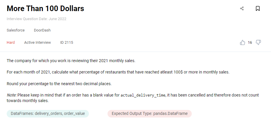
Link to the question: https://platform.stratascratch.com/coding/2115-more-than-100-dollars

Available data:

To solve this question, you need to work with data in two tables: delivery_orders and order_values.

Before answering the question, try to identify important values in each table. Let’s start with delivery_orders:

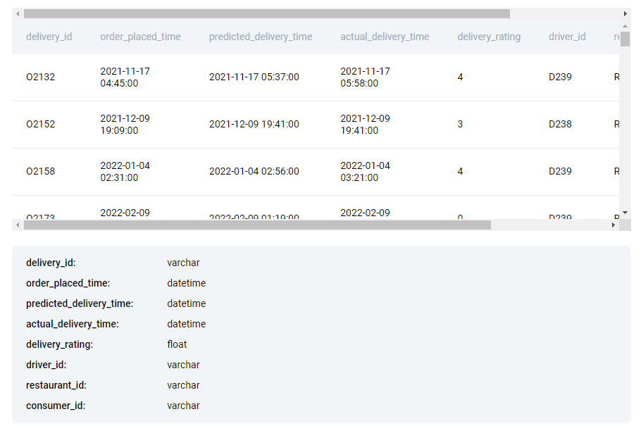
• delivery_id values are the shared dimension. We’ll use it to JOIN two tables.
• We need to find each restaurant’s monthly sales. It’s safe to assume that order_placed_time is going to be important.
• Most likely we won’t need values like predicted_delivery_time, actual_delivery_time, delivery_rating, delivery_rating, or dasher_id.
• We’ll use the restaurant_id value to aggregate sales for each restaurant.
• We don’t need to identify customers who placed the order, so consumer_id values can be ignored.

Now let’s look at the order_value table:

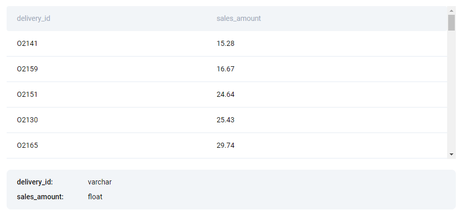
• We’ll use delivery_id values to JOIN two tables.
• sales_amount values represent delivery value in dollars.

Logical Approach

Solution to this question can be broken down into two steps:

1. Write a query that returns every restaurant’s monthly revenue.
2. For every month, find the percentage of restaurants that had at least $100 in sales.

To find every restaurant’s monthly revenue, we need to work with information from two tables. One contains information about deliveries (who prepared food, who delivered, at what time, and so on), and another contains information like each order’s dollar value. We’ll definitely need to JOIN two tables.

Also, it’s important to note that every row contains information about individual delivery. To get monthly sales for each restaurant, we'll need to aggregate records by month and restaurant_id.

Unfortunately, the table does not have a month value. In the SELECT statement, we need to use the EXTRACT() function to get months from the order_placed_time value and save it. Then use the GROUP BY statement to create groups for every restaurant in every month.

The question also specifies that we only need to work with deliveries completed in 2021. So we need an additional WHERE statement to set the condition. Once again, we use the EXTRACT() function to get the year from the order_placed_time value and make sure that it is 2021.

We also need to use the SUM() aggregate function to find total sales for each restaurant in each month. We can simply save total sales for each restaurant, but it’s much better if we use comparison operators (less than, or greater than) to compare the result of SUM() with 100 and save the result of a condition as a boolean.

In conclusion, a subquery that returns every restaurant’s monthly revenue will involve a fair bit of logic. It’s better to write this query outside of the main query, and save its result as a CTE.

With that, we have a query that calculates monthly sales for every restaurant.

To get the final answer, we’ll calculate the percentage of restaurants that met this threshold in each month.

We need to create groups for every month and use the AVG() aggregate function to calculate the percentage of restaurants with higher than $100 sales in that month.

As you may know, the AVG() function takes values from every record and then divides them by number of records to find the average. Our query does not contain total monthly sales for each restaurant, but a boolean that represents whether their sales were above 100.

Do you have an idea of how to use the AVG() function to find the ratio of true values in a certain column? Read our solution to find out how we did it.

Write the code

1. JOIN two tables

Information necessary to solve this question is split between two tables, so we need to combine them.

delivery_id is the shared dimension between them.

SELECT *
FROM delivery_orders d
JOIN order_value v ON d.delivery_id = v.delivery_id

One table contains information about deliveries, the other - about delivery values.

Both tables contain essential information - we don’t need delivery information without order values and vice versa. We should perform an INNER JOIN, which removes any deliveries without a match.

2. Filter deliveries by year

Tables contain delivery information for many years. The question explicitly tells us that we’re only interested in restaurant sales in 2021.

SELECT *
FROM delivery_orders d
JOIN order_value v ON d.delivery_id = v.delivery_id
WHERE EXTRACT(YEAR
              FROM order_placed_time) = 2021

Once we use INNER JOIN to combine two tables, we need to set an additional WHERE clause to filter deliveries by year.

There is no available data for the year when the order was placed, so we use the EXTRACT() function to get the year value from the order_placed_time value.

3. Find monthly sales for each restaurant

We use JOIN and WHERE to get information about all deliveries in 2021. Next, we must calculate monthly sales for each restaurant.

First, we use EXTRACT() to get the month from the order_placed_time value. This is the month when the order was placed. We use the AS command to give it a descriptive name. We can filter out canceled orders by checking if the actual_delivery_time is not null.

Next, we use GROUP BY to group records by unique pairs of restaurant_id and month values. Each group will have delivery records for each restaurant in each month.

Finally, we can use SUM() to add up sales_amount values for each group.

Technically, we could save total sales for each restaurant and later determine what percentage of these values is higher than 100. However, it’s better to get it out of the way now and simply store a boolean that represents whether monthly sales are above the $100 minimum.

SELECT restaurant_id,
       EXTRACT(MONTH
               FROM order_placed_time) AS month,
       SUM(sales_amount) > 100 AS above_100
FROM delivery_orders d
JOIN order_value v ON d.delivery_id = v.delivery_id
WHERE EXTRACT(YEAR
              FROM order_placed_time) = 2021
  AND actual_delivery_time IS NOT NULL
GROUP BY restaurant_id,
         month

As you can see, the query will return three values - restaurant_id, month, and above_100 boolean.

With that, we have a query that returns monthly sales for every restaurant. It’s fairly complex, so we should save it as CTE and simply reference the result.

4. Find the percentage of restaurants with over $100 in sales in each month

Query from step 3 returns all the information we need: restaurant id, monthly sales for that restaurant, and an above_100 value which represents whether or not those restaurants made at least $100 in sales. We will write it as a CTE.

Now we need to find what percentage of restaurants made more than $100 in sales. In other words, in each month, what percentage of restaurant records have above_100 values that are true.

The question tells us to output the month and share of restaurants with above $100 in sales.

At this point, each record represents a single restaurant in a month.

We’ll need to GROUP records by month and somehow calculate what percentage of above_100 values are true.

We can easily combine AVG() and CASE expressions to calculate this percentage.

The default behavior of AVG() is that it adds up all values in a group and divides the sum by the number of values to calculate the average. Instead, we can pass it a CASE expression that returns 1 if the above_100 is true and 0 if it’s false.

If there are 10 restaurants in a month, and only 3 have more than 100$ in sales, then AVG() will add up to 3, and divide it by 10, which gives us 0.3.

We multiply this ratio by 100 to get a percentage. As a cherry on top, we use the AS command to give it a descriptive name.

WITH cte AS
  (SELECT restaurant_id,
          EXTRACT(MONTH
                  FROM order_placed_time) AS month,
          SUM(sales_amount) > 100 AS above_100
   FROM delivery_orders d
   JOIN order_value v ON d.delivery_id = v.delivery_id
   WHERE EXTRACT(YEAR
                 FROM order_placed_time) = 2021
    AND actual_delivery_time IS NOT NULL
   GROUP BY restaurant_id,
            month)
SELECT month,
       100.0 * avg(CASE WHEN above_100 = True THEN 1 ELSE 0 END) AS perc_over_100
FROM cte
GROUP BY month;

This approach might seem unconventional, but CASE/WHEN is commonly used with aggregate functions.

Run the query to see if it matches the expected output for this question.

Output

The query should return the percentage of restaurants with over 100$ worth of sales in November and December.

Question 2: Completed Trip Within 168 Hours

Link to the question: https://platform.stratascratch.com/coding/2134-completed-trip-within-168-hours

Available data:

We are given two tables. Let’s take a quick look at values in the first:

• rider_id identifies the driver who signed up for the service. According to the question description, it corresponds with the driver_id value from the trip_details table. We’ll use it to JOIN two tables.
• Values in the event_name column will allow us to identify successful signups.
• timestamp values describe the time and date of the signup.

The trip_details table contains information about trips. Let’s look at important values in this table:

• driver_id identifies the Uber driver.
• actual_time_of_arrival specifies the time when the trip was complete.
• We’ll need to look at the status value to identify successful trips.
  

Logical Approach

To solve this question, we need to write two queries - one that returns all drivers who signed up in the first 7 days of 2022 and another that returns all drivers who completed a trip within 168 hours of signing up. Both of these queries are quite complex, so it’s best to save them as CTEs.

First, we create a query that returns all successful signups (all columns) in the first 7 days.

We filter the initial signup_events table to return only successful signups. We do that by using the LIKE operator and specifying the ‘su_success’ string.

Also, we use the AND and BETWEEN logical operators to specify the ‘acceptable’ range of dates: from ‘2022-01-01’ to ‘2022-01-07’. In other words, the first 7 days of 2022. Then we filter signup records by date. We use the DATE() function to get date values from the timestamp.

Next, we create a list of drivers who completed the trip within 168 hours of signing up.

Information about signup events and completed trips are stored in different tables, so first, we need to JOIN two tables. The question description tells us that the shared dimension between the two tables is rider_id and driver_id.

Then we need to filter the result of JOIN to meet these two conditions:

1. Trip must be completed
2. The time difference between time_of_arrival and the signup event is under 168 hours.
   

Since both conditions need to be met, we should use the AND logical operator to chain these two conditions and the WHERE clause to remove rows that don’t meet both conditions.

We can use the LIKE operator to make sure values in the status column match with the ‘completed’ string.

To find the difference and set a condition, simply subtract the time of the signup event (timestamp column) from the actual_time_of_arrival. However, this will not give us meaningful value. We need a difference in hours, so we must use the EXTRACT() function.

The answer would be more accurate if we get the difference in seconds first and divide the number of seconds by 3600 (the number of seconds in an hour). The first argument to the EXTRACT() function is the unit of time you want to extract. To get seconds, pass EPOCH.

We should use a comparison operator to return records where the result of division (seconds by 3600) is 168 or less.

If one driver completed multiple trips within 168 hours of signing up, he should still count as one driver. To achieve this, you should use a DISTINCT clause when you SELECT only unique driver_id values from the result of a JOIN.

Now we have a list of drivers who signed up in the first 7 days of 2022 and a list of drivers who completed a trip within 168 hours of signing up.

To answer this question, we need to find the ratio (and percentage) of drivers who completed a trip within 168 hours vs all drivers who signed up in the first 7 days.

We should use LEFT JOIN to retain all records of drivers who signed up in the first 7 days and partially fill in the information for drivers who did complete the trip in 168 hours. Then we can use COUNT() to get the number of all drivers who signed up in the first 7 days.

We also need another COUNT() to get the number of drivers who made their trip in the first 168 hours. Because of how LEFT JOIN works, some of these values will be NULL.

Finally, we need to divide the number of drivers who completed the trip in the first 168 hours by the larger number of drivers who signed up in the first 7 days. This will give us a ratio. Because the result is a float, we need to convert one of the results of a COUNT() function to a float as well.

To get the percentage, we multiply the ratio by 100.

Write the code

1. Write a query that returns all signups in the first 7 days

We need to filter the signup_events table to return successful signups in the first 7 days.

The table does not contain the date of the event. So we’ll use the DATE() function to get a date value from the timestamp value.

SELECT *,
       DATE(timestamp)
FROM signup_events
WHERE event_name LIKE 'su_success'
  AND DATE(timestamp) BETWEEN '2022-01-01' AND '2022-01-07'

Next, we’ll need to set up a WHERE statement and chain two conditions:

1. event_name value matches ‘su_success’ string
2. The date of the event falls between the 1st and 7th of January.

We use the BETWEEN operator to specify the date range.

The question asks us how many drivers who signed up in the first 7 days (the result of this query) completed the trip within 168 hours of signing up (the result of another query). Eventually, we’ll have to JOIN these two queries, so we should save it as CTE. Make sure to give it a descriptive name.

2. Write a query that returns all drivers who completed a trip within 168 hours

We need to JOIN two tables to get information about signup events and completed trips in one table.

We need to use the ON clause to define a shared dimension - rider_id value from the signup_events table and driver_id from the trip_details table.

SELECT DISTINCT driver_id
FROM signup_events
JOIN trip_details ON rider_id = driver_id
WHERE status LIKE 'completed'
  AND EXTRACT(EPOCH
              FROM actual_time_of_arrival - timestamp)/3600 <= 168

We chain an additional WHERE clause to set two conditions:

For each trip, the status value should match the ‘completed’ string and the time between signup event (timestamp) and actual_time_of_arrival is under 168 hours.

We use the EXTRACT() function to get the number of seconds between two timestamps. We specify EPOCH to get the number of seconds from the difference between two values.

Divide the result of the EXTRACT() function by 3600 to get the number of hours between two events. That number should be under 168.

Finally, we use the DISTINCT clause to make sure that each driver counts only once, even if they made multiple trips within 168 hours.

Save the result of this query as a CTE.

3. Find the percentage of drivers

We have a query that returns all drivers who signed up in the first 7 days and all drivers who completed the trip within 168 hours of signing up.

The question asks us how many drivers from the second list also appear in the first list. We should perform a LEFT JOIN, where the first table is signups (CTE that returns people who signed up in the first 7 days), and the second table is first_trips_in_168_hours (self-explanatory).

LEFT JOIN will keep all records from the first table but only the matching values from the second table.

SELECT city_id, date, CAST(COUNT(driver_id) AS FLOAT) / COUNT(rider_id) * 100.0 AS percentage
FROM signups
LEFT JOIN first_trips_in_168_hours ON rider_id = driver_id
GROUP BY city_id, date

Finally, we should find the percentage of drivers who meet the criteria in each city and date. Group records by city_id and date values.

To calculate the percentage, we use COUNT() to get the number of riders who completed a trip and divide it by the result of another COUNT() function, which finds the number of signups for each group.

The result should be a decimal value, so we convert the result of the COUNT() function to a float.

Finally, we multiply the ratio by 100 to get the percentage value and use the AS command to give it a descriptive name.

The complete query should look something like this:

WITH signups AS
  (SELECT *,
          DATE(timestamp)
   FROM signup_events
   WHERE event_name LIKE 'su_success'
     AND DATE(timestamp) BETWEEN '2022-01-01' AND '2022-01-07'),
     first_trips_in_168_hours AS
  (SELECT DISTINCT driver_id
   FROM signup_events
   JOIN trip_details ON rider_id = driver_id
   WHERE status LIKE 'completed'
     AND EXTRACT(EPOCH
                 FROM actual_time_of_arrival - timestamp)/3600 <= 168)
SELECT city_id, date, CAST(COUNT(driver_id) AS FLOAT) / COUNT(rider_id) * 100.0 AS percentage
FROM signups
LEFT JOIN first_trips_in_168_hours ON rider_id = driver_id
GROUP BY city_id, date

Try running the query to see if it matches the expected output.

Output

The output should include percentage values for each date and city.

Question 3: Above Average But Not At The Top

Link to the question: https://platform.stratascratch.com/coding/9985-above-average-but-not-at-the-top

Available data:

We are given one sf_public_salaries table. It contains a lot of values, but only a few are important.

• We don’t need to identify employees, we only output their names. So the id value can be ignored.
• The output includes employee names, so employeename values are necessary.
• We need to find the average salary for each jobtitle value.
• The totalpay column contains salary numbers.
• Other columns - base pay and benefits can be safely ignored.
• We’ll need to filter records by year.
• notes, agency, and status are not important.

Logical Approach

Answer to this question can be separated into two parts:

First, we write a query that finds the average pay for each job title in 2013. We'll have to group records by jobtitle value and use the AVG() function to find the average salary for each job title. Then chain an additional WHERE and set a condition - year should be equal to 2013.

To find employees with above-average salaries, we INNER JOIN this query with the main table on jobtitle, the shared dimension. We need INNER JOIN to remove rows that do not meet the criteria. We’ll use the ON clause to set the condition - employees must have above-average salaries.

We need INNER JOIN because it eliminates all rows that don’t meet the criteria.

To output the final answer, we need to filter records by one more condition - employees should not be among the TOP 5 earners for their job title. We’ll use window functions to rank employees and filter out the top 5 employees.

Then we should set an additional WHERE clause to filter the result of INNER JOIN. We should use the IN operator to record only the employee names that appear in the list of employees with a rank of 5 or below.

Write the code

1. Find average pay for job titles

The question asks us to return employees with above-average salaries. To do this, first, we need to find the average salary for each jobtitle in the year 2013.

SELECT jobtitle,
       AVG(totalpay) AS avg_pay
FROM sf_public_salaries
WHERE YEAR = 2013
GROUP BY jobtitle

We should group records by jobtitle value, and apply the AVG() aggregate function to totalpay column. Use the AS command to save the result of the AVG() function.

2. Filter out employees with below-average salaries

Next, we need to filter employees by their totalpay value.

We’ll use the avg_pay value as a minimum threshold. So we need to JOIN the main table with the result of the subquery that returns avg_pay.

In this case, we use the ON clause (instead of WHERE) to kill two birds with one stone: JOIN the main query and subquery on a shared dimension (jobtitle) and discard records of employees whose totalpay is below the avg_pay number.

SELECT main.employeename
FROM sf_public_salaries main
JOIN
  (SELECT jobtitle,
          AVG(totalpay) AS avg_pay
   FROM sf_public_salaries
   WHERE YEAR = 2013
   GROUP BY jobtitle) aves ON main.jobtitle = aves.jobtitle
AND main.totalpay > aves.avg_pay

Running this query will return all employees whose salary is above average for their position. However, the question tells us to exclude employees with TOP 5 salaries.

3. Get the list of employees who do not have the 5 highest salaries

We need a subquery that returns all employees, except those with the 5 highest salaries for their job title.

To accomplish this, first, we write a subquery that returns employeename, jobtitle, and totalpay values of employees. Also, we use the RANK() window function to rank employees by their salary (compared to others with the same jobtitle) and assign them a number to represent their rank.

Then we should SELECT employeename values of employee records where the rank value (named rk) is above 5.

SELECT employeename
     FROM
       (SELECT employeename,
               jobtitle,
               totalpay,
               RANK() OVER (PARTITION BY jobtitle
                            ORDER BY totalpay DESC) rk
        FROM sf_public_salaries
        WHERE YEAR = 2013 ) sq
     WHERE rk > 5

This subquery returns all employees who are NOT among TOP 5 earners for their job title.

4. Filter out the TOP 5 employees

In step 2, we had records of all employees with above-average salaries. The question tells us to exclude the Top 5 earners.

In step 3, we wrote a subquery that returns all employees except the TOP 5 earners.

So we need to set the WHERE clause to filter the initial list of employees with above-average salaries. We use the IN operator to return only the names of employees who:

1. Above average salary for their job title (filtered in the first JOIN)
2. Appear in the list of employees who are NOT top 5 earners for their position.

Final code:

SELECT main.employeename
FROM sf_public_salaries main
JOIN
  (SELECT jobtitle,
          AVG(totalpay) AS avg_pay
   FROM sf_public_salaries
   WHERE YEAR = 2013
   GROUP BY jobtitle) aves ON main.jobtitle = aves.jobtitle
AND main.totalpay > aves.avg_pay
WHERE main.employeename IN
    (SELECT employeename
     FROM
       (SELECT employeename,
               jobtitle,
               totalpay,
               RANK() OVER (PARTITION BY jobtitle
                            ORDER BY totalpay DESC) rk
        FROM sf_public_salaries
        WHERE YEAR = 2013 ) sq
     WHERE rk > 5)

Run the query to see if it returns the right answer.

Output

The query should return the name of the employee who meets both conditions - has above average salary, but not TOP 5 salary.

Question 4: Lyft Driver Salary and Service Tenure

Link to the question: https://platform.stratascratch.com/coding/10018-lyft-driver-salary-and-service-tenure

Available data:

We are given only one table with four columns. Let’s take a look at four columns:

• We won’t need index values, which are simply incremental numbers.
• To calculate the driver’s tenure, find the difference between start_date and end_date values
• We’ll use the yearly_salary value to find the correlation.

Logical Approach

To find the correlation, we need both yearly_salary and tenure values. We already have one and can find another by calculating the difference between start_date and end_date values.

The difficulty is that drivers still working for Lyft do not have an end_date value.

We can use the COALESCE() function to solve this problem. It returns the first non-NULL value. We can pass it two arguments - end_date and CURRENT_DATE, and subtract start_date from its result.

If there is a non-NULL end_date value, then COALESCE() will return end_date. If it’s NULL, COALESCE() should return the current date, and we’ll find the difference between it and start_date. We should use the AS command to describe the result of this operation.

Once we have both values, we can use the CORR() function to calculate correlation between tenure and salary.

Finally, we should SELECT tenure and yearly salary values and pass them as arguments to CORR() aggregate function. CORR() accepts numeric values, so when we generate tenure, we should cast it to a NUMERIC type.

Write the code

1. Calculate driver tenure

The table contains information about the driver's start_date and end_date, but not their tenure.

We calculate the tenure by finding the difference between end_date and start_date.

If the end_date is NULL (driver is currently driving for Lyft) then COALESCE() function will return today’s date (CURRENT_DATE). We will calculate the tenure by finding the difference between today’s date and start_date.

To make things easier, we should also SELECT yearly_salary and rename it to salary.

SELECT (COALESCE(end_date::DATE, CURRENT_DATE) - start_date::DATE)::NUMERIC AS duration,
       yearly_salary AS salary
FROM lyft_drivers

This subquery should return two values - driver’s tenure and their salary. We should save the result of this query as a CTE.

In the next step, we’ll find a correlation between salary and tenure. We can’t find a correlation between two values of different types, so we should cast tenure to a NUMERIC type.

2. Find the correlation between tenure and salary

At this point, we have a CTE that returns both tenure and salary values.

We only need to use the CORR() aggregate function to find a correlation between these two numbers. Correlation is going to be a decimal value, so we should cast it to a float type.

WITH df1 AS
  (SELECT (COALESCE(end_date::DATE, CURRENT_DATE) - start_date::DATE)::NUMERIC AS duration,
          yearly_salary AS salary
   FROM lyft_drivers)
SELECT CORR(duration, salary)::float
FROM df1

Run the query to see if it returns the right answer.

Output

The query should return only one value - a small decimal number to represent the correlation.

An error loading the results has occured

Question 5: Top 3 Wineries In The World

Link to the question:

https://platform.stratascratch.com/coding/10042-top-3-wineries-in-the-world

Available data:

All the necessary information is contained in one table.

• id value identifies each winery. It can be safely ignored.
• We need to find top wineries in each country, so country values are important.
• We also need to find average points for each winery.
• Our output should include winery names from the winery column.

Logical Approach

The first step should be calculating average points for wineries in each country. To achieve this, we need to group records by country and winery values and use the AVG() function to find average points for each group.

To avoid complexity, you should save the query as a CTE.

Next, you should rank wineries in each country by their points. You can use either ranking window functions like RANK(), or simply ROW_NUMBER(). If you order wineries in descending order (from highest points to lowest), you can use ROW_NUMBER() to assign numbers. So, the highest-scoring winery will be assigned number 1, the second-highest number 2, and so on.

The question tells us to order wineries by their names if average points are tied. The description also specifies the output format. It should have four columns: country and names* of corresponding first, second, and third-place wineries.

One important detail is that winery names should be followed by corresponding average points in parentheses (Madison Ridge (84) ).

The query to number rows can be quite complex. Better save it as CTE and reference its result.

Take a look at the expected output:

To achieve this, we need to use CASE/WHEN syntax in the SELECT statement to generate custom values for three columns. We’ll use the AS command to give three values descriptive names - top_winery, second_winery, and third_winery.

The CASE expression will look at position values to return values. If position is 1, then the CASE expression returns the respective name of that winery and concatenates three additional strings - an opening parenthesis, rounded average point value, and a closing parenthesis.

In SQL,  || is the concatenation operator.

Finally, we group records by country and use the MAX() aggregate function to return the highest, second-highest, and third-highest values in each group.

In some countries, there is only one winery so that that country won’t have second-place or third-place wineries. In this case, the question tells us to return ‘No second winery’ or ‘No third winery’.

We can use the COALESCE() function to handle this edge case. As you remember, it returns the first non-NULL value. We use the MAX() function to find the highest second_place value for each country. If that returns NULL, then COALESCE() will return specified strings - ‘No second winery’ for the second place or ‘No third winery’ for the third place.

Write the code

1. Average points for each winery

Each record in the winemag_p1 table contains wide-ranging information.

Before we rank wineries, we need to calculate the average points for each winery in each country.

So we SELECT these three values and write a GROUP BY statement to group records by country and winery.

In the SELECT statement, we use the AVG() aggregate function to find average points for each group.

SELECT country,
       winery,
       AVG(points) AS avg_points
FROM winemag_p1
WHERE country IS NOT NULL
GROUP BY country,
         winery

2. Rank wineries by their average points in each country

Next, we SELECT country, winery, and avg_points values from the subquery result and use the ROW_NUMBER() to rank wineries nationwide.

In this case, we order wineries within each country (partition) in descending order by their average points. Wineries with higher avg_points positioned first and followed by wineries with lower avg_points. We also specify that wineries with the same orders should be returned alphabetically.

ROW_NUMBER() assigns number values based on the records’ position in the partition. Because wineries are ranked by average points, ROW_NUMBER() effectively generates a number to represent the rank of each winery. We use the AS command to save its result as POSITION.

SELECT country,
       winery,
       ROW_NUMBER() OVER (PARTITION BY country
                                ORDER BY avg_points DESC, winery ASC) AS POSITION,
                               avg_points
      FROM
        (SELECT country,
                winery,
                AVG(points) AS avg_points
         FROM winemag_p1
         WHERE country IS NOT NULL
         GROUP BY country,
                  winery) tmp1

3. Generate top_winery, second_winery, and third_winery values

Next, we SELECT country values and use the CASE expression to create three values.

If the POSITION of a certain winery is 1, then CASE returns the name of the winery and concatenates average points placed between parenthesis.

The CASE expression that checks for wineries with a POSITION of 1 is named top_winery. Wineries with a POSITION value of 2 are named second winery, and POSITION value of 3 - third_winery.

If there are no wineries by positions 1, 2, or 3, our CASE expression returns NULL.

In SQL, we use the || operator to concatenate.

SELECT country,
          CASE
              WHEN POSITION = 1 THEN winery || ' (' || ROUND(avg_points) || ')'
              ELSE NULL
          END AS top_winery,
          CASE
              WHEN POSITION = 2 THEN winery || ' (' || ROUND(avg_points) || ')'
              ELSE NULL
          END AS second_winery,
          CASE
              WHEN POSITION = 3 THEN winery || ' (' || ROUND(avg_points) || ')'
              ELSE NULL
          END AS third_winery
   FROM
     (SELECT country,
             winery,
             ROW_NUMBER() OVER (PARTITION BY country
                                ORDER BY avg_points DESC, winery ASC) AS POSITION,
                               avg_points
      FROM
        (SELECT country,
                winery,
                AVG(points) AS avg_points
         FROM winemag_p1
         WHERE country IS NOT NULL
         GROUP BY country,
                  winery) tmp1) tmp2
   WHERE POSITION <= 3

We are not interested in wineries outside of TOP 3, so we set the WHERE clause to remove them.

4. Return the highest values or a placeholder

The question asks us to return the highest values by country. We should group records by country and use the MAX() aggregate function to find the highest top_winery score.

Next, we use the COALESCE() function to return the highest secondary_winery value. If a certain country does not have the second highest secondary_winery value, then COALESCE() returns a placeholder - ‘No second winery’.

Similarly, we use COALESCE() to return the highest third_winery value or a placeholder.

SELECT country,
       MAX(top_winery) AS top_winery,
       COALESCE(MAX(second_winery), 'No second winery') AS second_winery,
       COALESCE(MAX(third_winery), 'No third winery') AS third_winery
FROM
  (SELECT country,
          CASE
              WHEN POSITION = 1 THEN winery || ' (' || ROUND(avg_points) || ')'
              ELSE NULL
          END AS top_winery,
          CASE
              WHEN POSITION = 2 THEN winery || ' (' || ROUND(avg_points) || ')'
              ELSE NULL
          END AS second_winery,
          CASE
              WHEN POSITION = 3 THEN winery || ' (' || ROUND(avg_points) || ')'
              ELSE NULL
          END AS third_winery
   FROM
     (SELECT country,
             winery,
             ROW_NUMBER() OVER (PARTITION BY country
                                ORDER BY avg_points DESC, winery ASC) AS POSITION,
                               avg_points
      FROM
        (SELECT country,
                winery,
                AVG(points) AS avg_points
         FROM winemag_p1
         WHERE country IS NOT NULL
         GROUP BY country,
                  winery) tmp1) tmp2
   WHERE POSITION <= 3) tmp3
GROUP BY country

Run the query to see its result.

Output

The query should return three values: country, top_winery, second_winery, and third_winery. Not all countries will have second and third wineries. In that case, these columns should contain a placeholder.

Ten (Other) Strategies to Write Efficient and Advanced SQL Queries

In a professional environment, you need to write queries that are both correct and efficient. Companies often maintain millions of rows of data. Inefficient queries could lead to problems.

Let’s discuss 10 additional strategies for writing efficient queries.

1. SELECT column, not SELECT *

The SELECT statement should pull up essential values, nothing more. Don’t use an asterisk (*), which SELECTs all columns.

Queries always run faster on smaller volumes of data. Specifying columns also reduces the load on the database.

2. Use DISTINCT with caution

In SQL, deduplication is resource-expensive but often a necessary task. If you use DISTINCT, make sure it’s really necessary.

Also, use DISTINCT on values that uniquely identify the record. For example, if you want to remove duplicate records that describe the same person, apply DISTINCT to primary keys, not the name column. If you do make this mistake, DISTINCT might remove two different people with the same name.

3. Don’t use WHERE to combine tables

We can use the WHERE clause to combine tables conditionally. SELECT values from two tables, and set a WHERE clause to ensure these values are equal. Instead, use JOINs and the ON clause to combine tables on a shared dimension.

JOINs are specifically designed for combining tables in SQL. Not only are JOINs more efficient, but they are also more versatile than a simple WHERE statement.

4. Appropriate use of WHERE and HAVING

Both WHERE and HAVING clauses allow you to filter data in SQL. The big difference is that the WHERE clause filters records, whereas HAVING filters the results of aggregate functions.

In SQL, aggregation is an expensive operation. Your goal is to minimize the input to aggregate functions. If you need to filter records by certain criteria, use the WHERE clause to remove rows that do not meet the criteria, then group them and aggregate values in smaller groups.

This is more efficient than the alternative - group records in the entire table, apply aggregate functions to all rows and use HAVING to filter the results.

5. LIMIT to sample query results, look what your query outputs

Use LIMIT to see a reduced number of records from the output of the query. Looking at a limited sample lets you know if you need to change the query. More importantly, it puts less pressure on the production database.

6. Remove unnecessary ORDER BY

Ordering records in a resource-expensive operation. If you’re going to use ORDER BY, make sure it’s necessary.

Oftentimes ORDER BY is unnecessarily used in subqueries. If the main query uses ORDER BY, there’s no need to order rows in the subquery.

7. Reduce the cost of JOIN

You should always aim to reduce the size of tables before you JOIN them. Explore the possibility of removing duplicates or grouping records to reduce the number of queries in a table before you perform a JOIN.

8. Correct use of wildcards

Wildcards can be a useful tool for filtering text values. However, using wildcards to search the contents of the string can be expensive. If possible, try to use them only to evaluate the end of strings.

9. GROUP BY multiple columns

Sometimes, you must group records by two, three, or even more values. When you do, use the column with more distinct values first (id) and then the column with more common values (first name).

10. UNION vs UNION ALL

As we already mentioned, removing duplicates is an expensive operation. UNION vertically combines two datasets and takes the extra step of removing duplicate rows.

UNION ALL, on the other hand, combines the results of the queries and stops there. It is a much less expensive operation, so if your datasets do not contain duplicates or if duplicates are acceptable, UNION ALL is a more efficient choice.

Summary

In this article, we tried to explain advanced SQL concepts and their possible use cases. We also tried to demonstrate how to use them to answer Advanced SQL Questions modeled on data scientists’ actual day-to-day tasks.

Learning beyond basic SQL concepts allows you to choose the right feature (or combination of features) to write efficient and advanced SQL queries.

If you’d like to continue practicing advanced SQL concepts and features, sign up on the StrataScratch platform. Once there, you can explore hundreds of SQL interview questions of various difficulties, try to answer them, and read and participate in discussions about which SQL feature is best suited for the task.