Supervised vs Unsupervised Learning

 Written by:
Nathan Rosidi
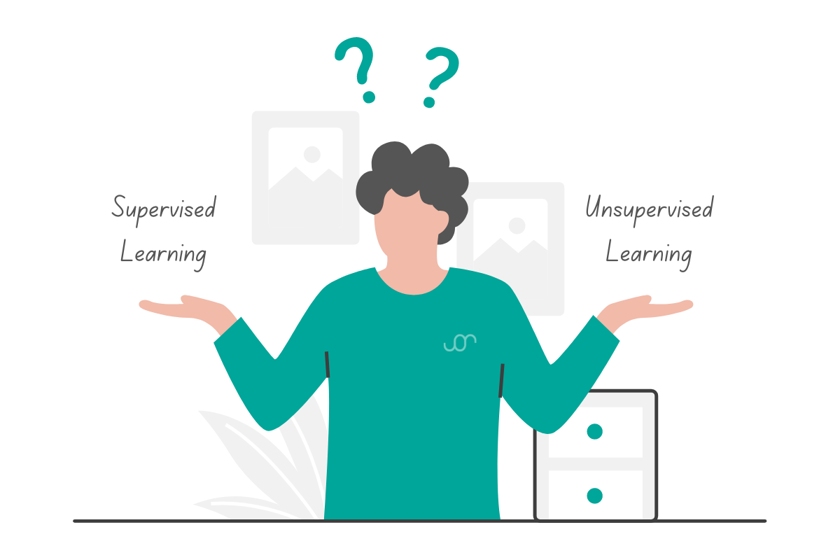
Supervised and unsupervised learning: the two approaches that we should know in the world of machine learning.
Supervised and unsupervised learning, both have their own strengths and usefulness, depending on their use cases. On the surface level, the most obvious difference between these two approaches is how the models within each approach are trained. However, there are a lot more things that differentiate the two approaches distinctively, and in this article of supervised vs unsupervised learning we’re going to discuss everything about these two approaches in a more detailed way soon.
In this article, we’re going to cover the following main points:
- Supervised learning: what supervised learning actually is and the algorithms that use the supervised learning approach
- Unsupervised learning: what unsupervised learning actually is and the algorithms that use the unsupervised learning approach
- The difference between supervised learning and unsupervised learning approach
- When should we use supervised learning and unsupervised learning approach
- Semi-supervised learning: the middle-ground between supervised and unsupervised learning approach
- The implementation of semi-supervised learning
Supervised vs Unsupervised Learning
Without further ado, let’s start with the first main talking point, which is the concept of supervised learning.
Supervised Learning
In a supervised learning algorithm, we need to provide the ground truth label for each data point during the training process of the model. There are two supervised learning algorithms that are commonly used in practice: regression and classification.
Regression
Regression is a machine learning algorithm that we can use when we want to predict continuous values, such as price, body weight, student’s grade, etc. Common examples of machine learning models for regression problems are:
Linear Regression
Linear regression is a machine learning algorithm that tries to capture the linear relationship between features and the continuous value that we want to predict. Let’s say you want to predict the price that you need to pay for a taxi. You can do so by first collecting data that shows the taxi price with respect to the corresponding travel distance. With linear regression, you’ll get the following result:


With the red line as shown above, you now can predict the price that you need to pay for your taxi just by looking at the travel distance to your final destination.
Polynomial Regression
Linear regression can produce more than just a straight line. And for this to happen, we need to transform the regression function from one degree to n degree, where n is the polynomial degree that we should define in advance.
Polynomial regression will be particularly helpful if we have non-linear data points, as it is able to produce a fitting line that captures the pattern of the non-linear data points, as you can see below:


Regularized Regression
Depending on the data points that we use for model training, the regression model that we built sometimes suffers from overfitting, which means that it tries to fit each of the data points way too hard, as you can see below:


This usually happens when our regression model is too complex. Regularized regression model adds additional terms in the regression equation to keep the weight small during the training process. Common regularized regression models are Ridge Regression, Lasso Regression, and Elastic Net.
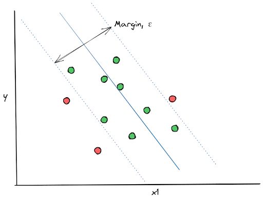
Support Vector Regression
Although this algorithm is more commonly used for classification algorithms, Support Vector Machine (SVM) can be used for regression use cases as well, and it’s normally called Support Vector Regression (SVR).
The main concept behind SVR algorithm is that the algorithm draws the best regression line that will fit the data points whilst also fulfilling the maximum margin, ε, that we define in advance, as you can see in the visualization below:

Decision Tree Regressor
Decision Tree is also another machine learning algorithm that is more commonly used for classification use cases, however it can be used for regression problems too.
There are three components in a decision tree algorithm: a root node, (normally) a bunch of interior nodes, and leaf nodes, as you can see in the visualization below:

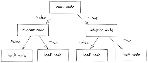
In each of the interior nodes, there is a True or False condition that each data point needs to fulfill to fully determine its final value. In a Decision Tree Regressor algorithm, the leaf nodes contain the prediction of the final continuous value of each data point.
Classification
Classification is a machine learning algorithm that we can use when we want to predict discrete values, such as whether an email is a spam or not, whether the sentiment of a tweet is positive or negative, whether an animal in a picture is a cat or dog, etc.
Since the value that we want to predict is discrete, then we can quantify the number of labels or ground-truth in our data, which leads to different types of classification problems, such as:
- Binary classification: if the label or ground-truth of our data consists only of two values, e.g cat or dog, positive or negative, pass or fail, etc.
- Multiclass classification: if the label or ground-truth of our data consists of more than two values, e.g {cat, dog, mouse, human}, {positive, negative, neutral}, {summer, winter, fall, spring}, etc
- Multilabel classification: if the label or ground-truth of our data consists of more than two values and the model can pick more than one label as the prediction.
Common examples of machine learning algorithms for classification use cases are:
Logistic Regression
The term ‘regression’ in logistic regression is not because it is a regression algorithm, but due to the fact that it uses the similar concept as linear regression, i.e the logistic regression uses a linear combination of the features in order to compute the cost function and optimize the weight.
Logistic regression uses a sigmoid activation function to map the outcome as probability with the range from 0 to 1, as you can see in the visualization below:

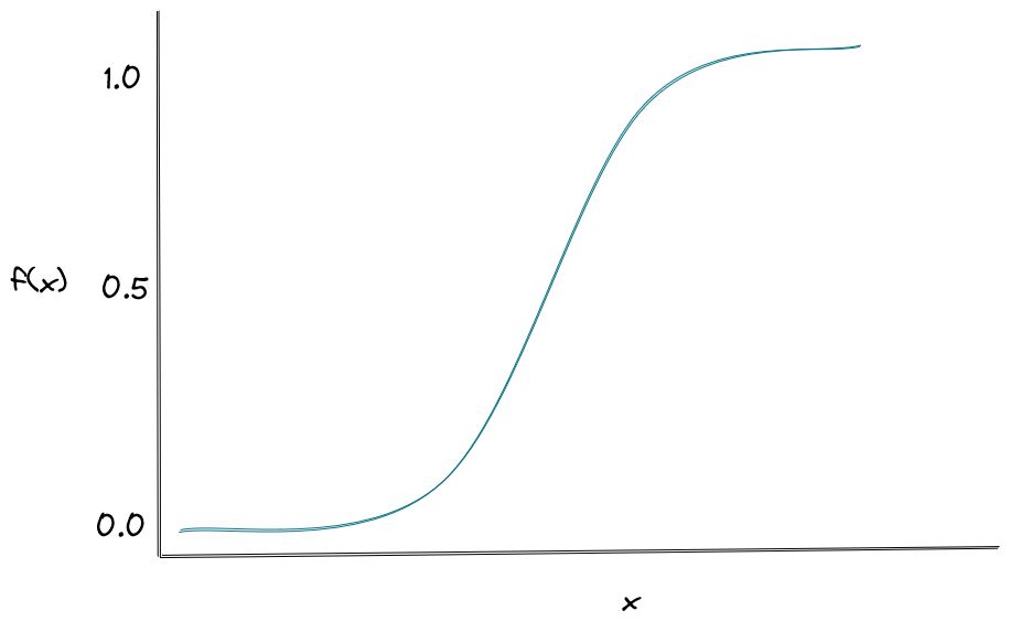
It’s normally used when we have a binary classification problem (i.e we only have two possible outcomes). Then, we make a prediction based on the value that comes from the sigmoid activation function above, i.e if the value is above 0.5, then we can classify a data point as 1 and if below 0.5, we can classify a data point as 0.
Softmax Regression
Softmax regression is the extension of logistic regression in the sense that it allows us to predict the outcome that has more than two possible outcomes. This is because unlike logistic regression which utilizes a sigmoid function, softmax regression utilizes a softmax function that computes the probability that each data point belongs to each label/class.
Support Vector Machine
Support Vector Machine (SVM) is a machine learning algorithm that is commonly used for classification problems, although it can be used for regression problems as well, as you can see in the previous section.
SVM works by generating a hyperplane in between two margin lines, as you can see in the visualization below:

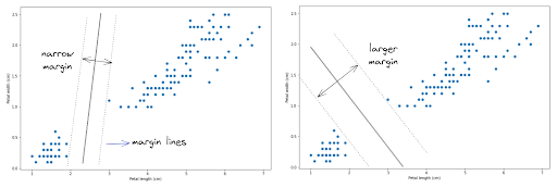
The main goal of the SVM algorithm is to generate the hyperplane with the widest possible margin to both of the margin lines, as you can see from the image on the right-hand side. The wider the margin, the better the hyperplane is in separating data points with different labels.
k-Nearest Neighbors
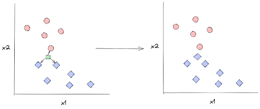
k-Nearest Neighbors (kNN) algorithm is a classification algorithm that works by keeping all of the training data in the memory even after the model has been built and trained. When we supply a KNN model with an unseen data point, first it will look at its surrounding k nearest neighbors. This value k is the hyperparameter that we should define in advance.
Let’s say that we set the value of k to 3. When we supply the model with a new data point, the model then will first determine three of its closest neighbors and then that new data point will be assigned a label according to the majority label of its three chosen neighbors, as you can see in the visualization below:

Decision Tree
Decision Tree is a tree-based algorithm with the same concept as you have seen in the Decision Tree Regressor above.
It consists of a root node, a bunch of interior nodes, and leaf nodes. There is a True or False condition in each level of interior nodes that each data point needs to fulfill.
The difference between the Decision Tree for classification and regression is the value that we’re going to get in each of the leaf nodes. As you might have guessed, in classification problems, the value of the leaf nodes is discrete and vice versa, it’s continuous in regression problems.
Ensemble Method
We’ve seen that there are several machine learning algorithms that we can use for classification problems, but what if we use several of them and then combine their predictive power at the end? This is the idea behind the ensemble method. There are several approaches for ensemble methods, such as:
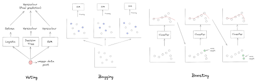
- Voting: We use several machine learning algorithms to predict the same thing, and at the end, the prediction of each machine learning algorithm is aggregated to form the final prediction
- Bagging: We use several machine learning models consisting of one particular algorithm, let’s say a Decision Tree, but each of them is trained with a different subset of training data. In the end, the prediction from each model is aggregated.
- Boosting: We train several models sequentially in order to transform several weak models into one strong model. Two algorithms are commonly used in the real-life problem that uses Boosting at their core: AdaBoost and Gradient Boosting

If you want to learn each of the algorithms mentioned above in a deeper sense, you can read the overview of machine learning algorithms for regression problems and the overview of machine learning algorithms for classification problems.
Unsupervised Learning
So far we have covered the concept of supervised learning as well as common machine learning algorithms for both regression and classification problems. Now let’s talk about the second approach in the whole spectrum of machine learning, which is unsupervised learning.
In contrast with supervised learning, we don’t need to provide the model with the ground truth label of each data point during the training process. This means that the model will learn the pattern of data points by itself, hence the name ‘unsupervised’.
In real life application, unsupervised learning is a very useful method since most of the data are unlabeled and the fact that it’s very time consuming to provide a ground-truth label for each data point.
There are a lot of examples of use cases that use the unsupervised learning approach, such as dimensionality reduction, clustering, and anomaly detection.
Dimensionality Reduction
Dimensionality reduction is an approach that we use to alleviate the so-called the curse of dimensionality problem.
The curse of dimensionality problem often occurs when we have tons of predictors when we want to train a machine learning model for classification or regression purposes. When we have tons of features, the latent space would be very sparse and thus, makes the prediction of our trained model become less reliable.
Another useful thing about dimensionality reduction is that it allows us to visualize high dimensional data in 2D or 3D. Common machine learning models for dimensionality reduction are:
Principal Component Analysis
Principal Component Analysis (PCA) is an algorithm mainly used for dimensionality reduction. It tries to project high-dimensional data into its lower-dimension representation by projecting the data into the axes that preserve the variance of our dataset the most.

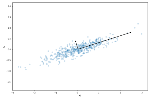
The axes chosen by the PCA algorithm are called principal components, as you can see from the two black lines above. Once all of the principal components have been identified by the algorithm, then we can observe how big is the variance of our original dataset that has been preserved by each principal component.
t-SNE
t-distributed Stochastic Neighbor Embedding is a nonlinear dimensionality reduction technique that aims to reduce the dimension of high-dimensional data based on the density between a data point with its neighbor with the student-t distribution.

The set of probabilities between each data point to its neighbors in the high dimension will then be mapped into the lower dimension with Kullback-Liebler (KL) divergence. This KL divergence should be optimized with a gradient descent algorithm.
Locally Linear Embedding
Locally Linear Embedding (LLE) is a nonlinear dimensionality reduction technique that works by first identifying the n closest neighbors of each data point. Let’s say that we have a data point x, LLE then tries to identify its n nearest neighbors, and then reconstruct data point x as a linear function of its n nearest neighbors.
In common practice, there are three alternatives or improvements from the standard LLE, which are:
- Modified LLE: this algorithm is designed to solve the regularization problem of the regular LLE algorithm by applying multiple weight vectors in each neighborhood
- Hessian LLE: this algorithm uses Hessian-based quadratic form in each neighborhood to solve the regularization problem of the regular LLE algorithm
- Linear Tangent Space Alignment (LTSA): This algorithm uses the tangent space instead of regular distance to recognize the local geometry in each neighborhood
Clustering
Clustering is an approach that we normally use when we want to group data points into clusters. For example, whenever we want to cluster our customers into groups such that we can create a better, personalized product recommendation for each of them.
Below are common machine learning algorithms for clustering.
k-Means Clustering
k-Means clustering is one of the most used clustering algorithms out there. It uses an iterative approach to cluster our dataset. As a first step, we need to define the number of centroids (clusters) and these centroids will be initialized randomly in the search space.


In each iteration, there are two important steps applied in k-means clustering
- Each data point is assigned to the nearest centroid.
- The centroid position then will be moved according to the center of all of the data points assigned to it.
The two steps above will be conducted iteratively until the solution converges.
DBSCAN
DBSCAN is a clustering method that works by estimating the neighborhood density of each data point. In general, there are four steps in how DBSCAN is conducted:
- First, we need to define the distance between two data points that will be counted as a neighbor (let’s call this ε)
- Next, the number of neighbors of each data point based on the ε value is counted.
- If the number of neighbors exceeds a threshold value, then any particular data point will be turned into a core sample by the DBSCAN algorithm
- All of the neighbors of a core sample will be clustered into one group.
HDBSCAN
HDBSCAN or Hierarchical DBSCAN is an extension method for the DBSCAN clustering method above. The difference is that with HDBSCAN, we don’t need to specify the ε value in advance, as the HDBSCAN algorithm is designed to implement the DBSCAN algorithm with varying distances.
Gaussian Mixture Model
Gaussian Mixture Model is an algorithm that is commonly used for a number of applications within an unsupervised learning domain, such as clustering and anomaly detection. In a nutshell, here are the steps of how Gaussian Mixture Model works:
- We define the number of Gaussian distributions there is in our Gaussian Mixture Model. The number of Gaussian distributions will be equal to the number of clusters, each with its own mean and variance.
- The location of each data point then will be approximated by the Gaussian distribution from a random cluster with a particular mean and variance.
Gaussian Mixture Model is a probabilistic model in which it assumes that our data points are generated from several Gaussian distributions with unknown parameters.
Anomaly Detection
Anomaly detection is an approach to identify a few data points that deviate significantly from the rest of the data points. The main applications for anomaly detection include fraud detection of credit card usage, hacking prevention of websites, etc.
Common machine learning models for anomaly detection are:
Gaussian Mixture Model
As mentioned above, Gaussian Mixture Model can also be used for anomaly detection. However, the concept of using Gaussian Mixture Model for anomaly detection is different from the one in clustering.
The concept for using Gaussian Mixture Model for anomaly detection itself is pretty simple. If a data point is located in the low-density region after being approximated by Gaussian distribution, then we can consider that particular data point as an outlier or anomaly. We can set a threshold value in advance and set it accordingly in order to adjust false-positive and false-negative results.
Isolation Forest
From the name itself, you might have already guessed that this algorithm is a tree-based method, just like the Decision Tree that we use in the supervised learning technique. The concept behind Isolation Forest is that the data point that can be considered as an outlier or an anomaly normally would be placed much closer to the root node compared to the normal data points.

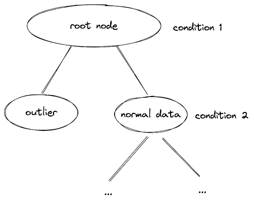
The tree-based method consists of a root node, several interior nodes, and leaf nodes. In each branch of the interior node, there will be a True or False condition that each data point needs to fulfill. If a data point is an outlier, then it will be located in the interior nodes close to the root node.
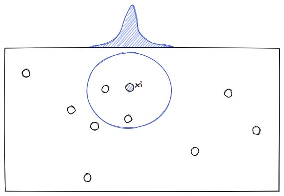
Local Outlier Factor
Local Outlier Factor is another unsupervised learning algorithm that works similarly to the k-Nearest Neighbors (kNN) algorithm that we’ve seen in the supervised learning algorithm.
In the kNN algorithm, we try to predict the ground-truth label of an unseen data point based on the majority label of its k-nearest neighbors.


In the Local Outlier Factor, the concept is similar. This algorithm tries to compute the so-called reachability of each data point to its k-nearest neighbors. The reachability is the distance between a data point to each of its neighbors. If the average travel distance of a data point to each of its neighbors is large, then that particular data point will be considered an anomaly or an outlier.
If you want to learn each of the algorithms mentioned above in a deeper sense, you can read the overview of machine learning algorithms within unsupervised learning domain.
Difference Between Supervised and Unsupervised Learning
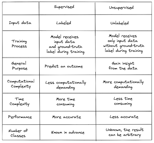
As mentioned previously, the most obvious difference between supervised and unsupervised learning is how the models are trained: one with the ground-truth label and one without.
However, there are other key differences between supervised learning and unsupervised learning:
- With supervised learning, you normally want to build a machine learning model with the end goal to predict something, for example the house price, the sentiment of a tweet, the class of an image, etc. Meanwhile, with unsupervised learning, the end goal of a machine learning model is to gain insight from our data.
- With supervised learning, we can train a machine learning model with a limited amount of data and still achieve a great result. However, that’s often not the case with an unsupervised learning approach. Unsupervised learning is more complex computationally because we need a large amount of data to achieve a meaningful result.
- With supervised learning, it can be time-consuming to train a model because we need to label our data beforehand, especially when we have a big dataset. Moreover, it requires expertise in a particular subject in order to accurately label each of the data points. Meanwhile in unsupervised learning, we don’t need to spend a lot of time training the model as we don’t need to provide the label of each data, but the result might be highly inaccurate and it needs human decision to assess the quality and the performance of the model.
If you need point-by-point differences between supervised and unsupervised learning, you can take a look at the table below:

Supervised vs Unsupervised Learning: Which of these two machine learning approaches we need to use?
Now the question is: which of these two machine learning approaches that we need to use? Well, it depends on the use case that we’re trying to solve.
If our end goal is to build a model to predict an outcome, the supervised learning approach would be more appropriate since it will give us quantifiable metrics that we can track in terms of its performance. If you have a large dataset and want to gain insight into your data, then an unsupervised learning approach would be more appropriate.
However, there is an approach that can act as a middle-ground between supervised learning and unsupervised learning, which is called the semi-supervised learning approach. We’ll discuss semi-supervised learning in more detail in the next section.
Semi-supervised Learning
Semi-supervised learning is a method that bridges the gap between the supervised learning approach and the unsupervised learning approach. As we can call this a ‘middle ground’ approach, then it can mitigate the drawbacks of both supervised and unsupervised learning, but it won’t perform as good as supervised and unsupervised learning in terms of their strength.
Nevertheless, this approach is very useful because as you already know, labeling data is a time-consuming process and the unfortunate reality is most of the real-world data is unlabeled. The good news is the algorithm with a semi-supervised approach can handle partially labeled data.
Semi-supervised model normally consists of a combination of a supervised learning model and an unsupervised learning model. As an example, a semi-supervised model can be a combination of logistic regression (supervised learning) and the k-means clustering method (unsupervised learning). Alternatively, we can turn a supervised learning classifier into a semi-supervised learning classifier, allowing it to learn from partially labeled data.
In the next section, you’ll see an example of how we can implement a semi-supervised learning approach on the iris dataset.
Semi-Supervised Learning: Implementation
In this section, we will implement a semi-supervised learning algorithm on the iris dataset. Specifically, we’re going to build a model that is based on a Support Vector Machine (SVM) as our classifier (supervised learning approach).
We’re going to compare the performance of the SVM model as a pure supervised learning algorithm with the SVM model after we turn it into a semi-supervised learning algorithm.
In general, there are two approaches to how we can implement a semi-supervised learning approach: with self-training method and with label propagation method. First, let’s take a look at the Self-training method first.
Self-Training Method
Self-training method is a ‘trick’ to turn our supervised learning model into a semi-supervised learning model. The only prerequisite is that we need to use a supervised learning model that produces a probability in its prediction.
It’s very straightforward to explain how self-training method works:
- First, we gather the whole dataset, a mixture of labeled and unlabeled data. But we only train our supervised learning model with the labeled data.
- The trained model will then make predictions of unlabeled data. The prediction will be the probability of an unlabeled data point belonging to each class.
- If the probability of an unlabeled data point belonging to a particular class is high (for example above 95%), then we use the predicted label as the label of this unlabeled data point.
- Next, we train our model again with these newly added labeled data and then make predictions again.
- The steps above are repeated until either one of these conditions is fulfilled: all of the data are labeled, no additional unlabeled data satisfy the probability threshold, or it reaches the maximum iteration step.
We can implement a self-training approach with the scikit-learn library easily. In the code snippet below, the base classifier, which is a Support Vector Classifier, will be trained on a fully labeled dataset and then its decision boundary will be compared with its self-training representation (i.e only trained on 30 and 50 labeled data instead of the whole dataset).
import numpy as np
import matplotlib.pyplot as plt
from sklearn import datasets
from sklearn.svm import SVC
from sklearn.semi_supervised import SelfTrainingClassifier

iris = datasets.load_iris()

X = iris.data[:, :2]
y = iris.target

rng = np.random.RandomState(0)
y_rand = rng.rand(y.shape[0])

# set random samples to be unlabeled
y_30 = np.copy(y)
y_30[y_rand < 0.3] = -1
y_50 = np.copy(y)
y_50[y_rand < 0.5] = -1


# the base classifier for self-training is identical to the SVC
base_classifier = SVC(kernel="rbf", gamma=0.5, probability=True)

# fit self-training with 30 labeled data
st30 = (
   SelfTrainingClassifier(base_classifier).fit(X, y_30),
   y_30,
   "Self-training 30% data",
)

# fit self-training with 50 labeled data
st50 = (
   SelfTrainingClassifier(base_classifier).fit(X, y_50),
   y_50,
   "Self-training 50% data",
)

# fit base classifier
rbf_svc = (SVC(kernel="rbf", gamma=0.5).fit(X, y), y, "SVC with rbf kernel")
And if we plot the decision boundary of each of the classifiers, we will get the following visualization:

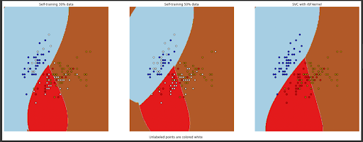
As we can see, both self-training models that have been trained on only 30 and 50 labeled data points can give us a decision boundary that is comparable to the model that has been trained on the full dataset.
Label Propagation
With label propagation, we don’t turn our supervised model into a semi-supervised model per se, but rather it’s an algorithm where we can turn our unlabeled data into labeled data. It works by connecting the whole dataset based on their distance, which typically is computed with Euclidean distance.
Label propagation treats a dataset as a graph, where each data point can be seen as a node, and the edge connecting two nodes can be seen as the notion of similarity between them (distance between two nodes). If the distance between two nodes is small, then it can be inferred that the two nodes have the same label and vice versa.
It’s also very simple to implement Label Propagation with the scikit-learn library. In the code snippet below, we will do the same as the one in the self-training method above. First, we have a base classifier, which is a Support Vector Machine, that will be trained on the fully labeled dataset. Then, the decision boundary of this base classifier will be compared with the decision boundary of two models that will be trained on the dataset labeled with the label propagation method.
One model will be trained on a dataset with label propagation from 30 labeled data, and another will be trained on a dataset with label propagation from 50 labeled data.
import numpy as np
import matplotlib.pyplot as plt
from sklearn import datasets
from sklearn.svm import SVC
from sklearn.semi_supervised import LabelPropagation

iris = datasets.load_iris()

X = iris.data[:, :2]
y = iris.target

rng = np.random.RandomState(0)
y_rand = rng.rand(y.shape[0])

# set random samples to be unlabeled
y_30 = np.copy(y)
y_30[y_rand < 0.3] = -1
y_50 = np.copy(y)
y_50[y_rand < 0.5] = -1

# fit label propagation with 30 labeled data
ls30 = (LabelPropagation().fit(X, y_30), y_30, "Label Propagation 30% data")

# fit label propagation with 50 labeled data
ls50 = (LabelPropagation().fit(X, y_50), y_50, "Label Propagation 50% data")

# fit base classifier
rbf_svc = (SVC(kernel="rbf", gamma=0.5).fit(X, y), y, "SVC with rbf kernel")
If we plot the decision boundary of each of the classifiers above, we’ll get the following visualization plot:

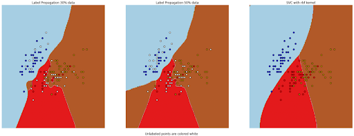
As you can see, both models that have been trained on a dataset with the label from the label propagation method perform reasonably well and created a similar boundary decision compared to the model that has been trained on a fully labeled dataset.
Conclusion
In this article, we learned about two main paradigms in the machine learning domain: the supervised learning method and the unsupervised learning method. Specifically, we now know which algorithms can be classified as supervised and unsupervised methods, the difference between supervised vs unsupervised learning, as well as the advantages and disadvantages of supervised and unsupervised learning methods.
Moreover, we also learned about semi-supervised learning, which can be seen as the middle ground between supervised and unsupervised learning methods. Semi-supervised learning proves to be a very useful method in a use case where we have a lot of unlabeled data, but don’t have time to label all of the data, whilst keeping the performance of the machine learning model reasonably well in comparison to the supervised learning model.
Share