SQL Window Functions Interview Questions


Categories:
 Written by:
Nathan Rosidi
Here’s an article to help you answer the SQL interview questions that require knowledge of the SQL window functions.
If you want to work in data science – and you wouldn’t be reading this if you didn’t – you have to be proficient in at least two areas: SQL and job interviews. Yes, both are skills that require practice.
When we say SQL, this is an area so broad that even its creators probably wouldn’t know everything about it. There’s no point in telling you that you should learn the ‘whole’ SQL to get a job as a data professional. Why? Because you don’t have to! Go cycling, swimming, read a book. Staring at the wall and watching paint dry is a better spent time than learning the ‘whole’ SQL.
What you need is a strong knowledge of some SQL concepts. The ones you’ll use in practice. The window functions are one of them. The interviewers like them, and you’ll like them, too, because they truly will make your day-to-day job easier.
And what about the job interviews? How is that a skill? Isn’t that just a dreadful event you have to experience to get a job? Yes, it is. But it’s not only that! When we talk about it being a skill, we mean having a clear approach to answering the SQL questions.
Writing the correct SQL code is important, don’t get us wrong. But having an outlined framework for solving the interview questions is equally important. And this is not a euphemism. Have a good framework, and you’ll easier write flawless code. Even if you f*** it up, and everybody sometimes does, you’ll get the points for your process and way of thinking.
What Are the SQL Window Functions, Anyway?
You don’t know already? No worries, there’s a SQL Window Functions guide where you’ll learn more than you want to know.
For those of you who are already familiar with the window functions, a short reminder before we go to solving the SQL window functions interview questions.
The window functions are usually seen as the more posh version of the SQL aggregate functions. The aggregate functions, you know that already, take values from multiple rows and return one value. Yes, this is data aggregation. The most popular aggregate functions are SUM(), COUNT(), AVG(), MIN(), and MAX().
They are often used in the GROUP BY clause. That way, data can be aggregated on multiple columns, which extends the aggregate functions’ analytical possibilities.
However, they still don’t retain the individual rows that are the basis for aggregation. The window functions do, and that is the main difference between the two! In other words, the SQL window functions allow you to aggregate data and show the analytical background behind the aggregation.
But, the window functions are even more than that. They are broadly divided into three categories:
- Aggregate Window Functions
- Ranking Window Functions
- Value Window Function
You can read all about them in the above guide. We’re here to show you the practical examples, not bore you to death with theory. So let’s set up our approach to solving the SQL window functions interview questions and see how it can be applied to the questions testing your window functions knowledge.
How to Approach SQL Window Functions Interview Questions?

The only thing that makes up the ‘right’ approach to solving the questions is making it structured. All other things are less relevant. The approach will vary from person to person and will be based on how you think and what approach you feel comfortable with.
Our approach that is proven successful consists of the following steps.
- Exploring the dataset
- Identifying columns for solving the question
- Writing out the code logic
- Coding
1. Exploring the Dataset
The interview questions usually have a concrete dataset you should use to come up with a solution.
The data is set up in a way that it tests certain SQL concepts. Always take some time to get to know the data types and inspect data for duplicates, NULL values, or missing values. This all influences your code and the functions you have to use.
If there is more than one table, inspect how the tables are interconnected, how you could join them, and which JOIN you should use.
This is not always possible, but when it is, preview the data itself. It will help you get a clearer picture and maybe find something you could have missed by only looking at the column names and data types.
2. Identifying Columns for Solving the Question
Less is not more, but it’s usually enough! Most questions will give you more data than you need to write a solution. Use this step to get rid of the columns you don’t need and write down the columns you do.
3. Writing Out the Code Logic
This literally means how it sounds: divide the code into logical blocks and write them down as steps. Usually, the ‘logic’ refers to the functions you’ll use. Number the steps, write down the function, and shortly describe how and why you’ll use it.
You can also write a pseudo code if you want, which you will just fill in with the actual data from the interview question.
As you’re writing the code logic, use this step to check with the interviewer to see if you’re moving in the right direction. Once you have the code logic written out, coding will be almost a technicality.
4. Coding
Most of the thinking was done in the previous steps. This will make code writing much easier because you’ll have most of the issues thought out already. Now you can focus on writing efficient code and have more bandwidth to tackle anything that comes up.
Window Functions in the SQL Interview Questions

Now, something that you’ve all been waiting for: solving the actual SQL window functions interview questions!
Question #1 Aggregate Window Function: Average Salaries
Creating an analysis similar to the one required by Salesforce is very usual, and it’s a perfect example of how similar and different the window functions are compared to the aggregate functions.


Link to the question: https://platform.stratascratch.com/coding/9917-average-salaries
Solution Approach
1. Exploring the Dataset
You’re given a table employee with the following columns and data types.
| id: | int |
| first_name: | varchar |
| last_name: | varchar |
| age: | int |
| sex: | varchar |
| employee_title: | varchar |
| department: | varchar |
| salary: | int |
| target: | int |
| bonus: | int |
| email: | varchar |
| city: | varchar |
| address: | varchar |
| manager_id: | int |
This is a fairly standard table with data about the company’s employees. We’re mostly interested in their salaries, and there are two possibilities how the table could record this data:
- Showing historical salaries
- Showing the latest actual salary
The first case would mean the employees and all other data could be duplicate, with different salary values for the same employee.
The second option is that there are no duplicate employees here, i.e., each employee appears only once.
We don’t know, but we can ask the interviewer or, even better, preview the data in the table.
This preview shows only several first rows, but believe me when I tell you there are no duplicates. This is an important thing to know. We now know we don’t have to remove the duplicates to ensure the salary data is not skewed by including one employee several times.
2. Identifying Columns for Solving the Question
This SQL window functions interview question gives a straightforward instruction about which columns you should output:
- department
- first_name
- salary
It also asks to show the average salary by department. To get that, we will again use the salary column. You can disregard all other columns.
3. Writing Out the Code Logic
The solution can be divided into two steps:
- SELECT columns from the table employees – department, first_name, salary
- AVG() as the window function – to get the average salary by department
4. Coding
All that remains to be done is translate the two steps into an SQL code.
1. SELECT Columns
SELECT department,
       first_name,
       salary
FROM employee;
2. AVG() Window Function
By completing the second step, you get the final code.
SELECT department,
       first_name,
       salary,
       AVG(salary) OVER (PARTITION BY department)
FROM employee;
The column salary is an argument in the AVG() function. However, we want to output the average salary by department, which requires the window function.
The window functions are always called by the OVER() clause. One of the optional clauses is PARTITION BY. Its purpose is to divide data into subsets that we want the window function to apply to. In other words, if data is partitioned by the column department, the window function will return the average salary by department.
Run the code in the widget to get the below output.

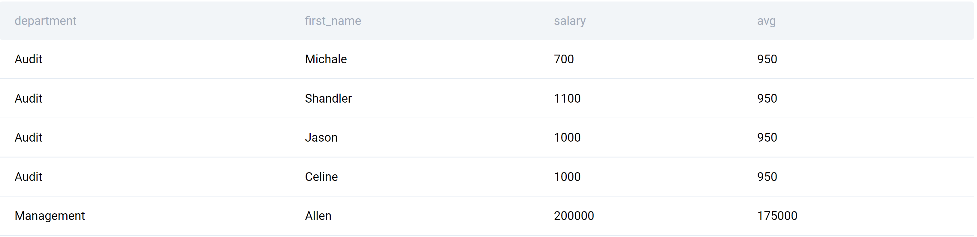
By only using the aggregate function, you wouldn’t have been able to show the analytical data and the department average at the same time. This is the power of the window functions!
Here, the output shows each employee and their salary along with the corresponding department average salary. you could go even further and analyze which employees are above and below the average of the department or a company. That way you can decide on adjusting the salaries to be more fair.
Question #2 Ranking Window Function: Best Selling Item
The aggregate window functions do the same as the ‘regular’ aggregate functions, except with more sophistication.
The SQL ranking functions, however, go even further than that. They give you the possibility to rank data, something that the aggregate function can’t do.
Working with data means you’ll do a lot of ranking. In business, creating reports that shows data such as top sales, revenue periods, or best selling item is almost a daily request.
The question by Amazon reflects this.

Link to the question: https://platform.stratascratch.com/coding/10172-best-selling-item
Solution Approach
1. Exploring the Dataset
The dataset, again, consists of only one table: online_retail.
| invoiceno: | varchar |
| stockcode: | varchar |
| description: | varchar |
| quantity: | int |
| invoicedate: | datetime |
| unitprice: | float |
| customerid: | float |
| country: | varchar |
The fair assumption would be that this is a list of online orders. The invoice numbers are probably unique, while other data can be duplicate.
This is confirmed by the data overview.
If you take a look at the whole table, you’ll realize that all the columns except invoiceno have duplicate values. This is expected, because one customer can place multiple orders, also of the same product and in the same quantity and unit price, even on a same date. We can distinguish these orders by the column invoiceno.
Of course, it can also happen that several different orders from different customers are the same. The columns invoiceno and customerid are there to distinguish between them.
Also, the best selling item is calculated by multiplying the quantity with the unit price. The unit price is a float data type, which means we don’t need to convert any data before multiplying.
2. Identifying Columns for Solving the Question
The instructions are to output the item description and amount paid.
We need to find the best selling item each month. The sales are the quantity multiplied by the price. As for the month, we have invoicedate column for that.
All this means we need the following columns to solve the problem.
- description
- unitprice
- quantity
- invoicedate
3. Writing Out the Code Logic
This is one of the hard SQL window functions interview questions that requires more steps than the previous one.
- SELECT the description FROM the table online_retail
- DATE_PART() – to get months from invoicedate
- SUM(unitprice * quantity) – to get the total amount paid
- RANK() window function – to rank the total amount paid for each month
- GROUP BY – to get data by month and by item description
- Subquery ��– write it as a subquery in the FROM clause
- SELECT month, description, and amount paid from the subquery
- WHERE clause – to show only the best selling in each month
4. Coding
1. SELECT Description FROM the Table
SELECT description
FROM online_retail;
2. DATE_PART()
Use the DATE_PART() function on the column invoicedate to show the month.
SELECT DATE_PART('month', invoicedate) AS month,
       description
FROM online_retail;
3. SUM()
By multiplying the quantity with the item price, you will get total sales. Then sum all the sales of the same item from the same month.
SELECT DATE_PART('month', invoicedate) AS MONTH,
       description,
       SUM(unitprice * quantity) AS total_paid
FROM online_retail;
4. RANK() Window Function
The data has to be ranked according to the month. Since SQL doesn’t allow referencing the column alias in this case, we’ll again have to use the DATE_PART() function in the PARTITION BY clause.
Another optional clause in OVER() is ORDER BY. We are ranking the data by the column total_paid. This, again, is an alias, so we need to use the whole formula. We sort the data within partition from the highest to lowest total paid amount.
SELECT DATE_PART('month', invoicedate) AS month,
       description,
       SUM(unitprice * quantity) AS total_paid,
       RANK() OVER (PARTITION BY date_part('month', invoicedate)
                    ORDER BY SUM(unitprice * quantity) DESC) AS rnk
FROM online_retail;
5. Group Data
For this part of code to work, data needs to be grouped by month and description.
SELECT DATE_PART('month', invoicedate) AS month,
       description,
       SUM(unitprice * quantity) AS total_paid,
       RANK() OVER (PARTITION BY date_part('month', invoicedate)
                    ORDER BY SUM(unitprice * quantity) DESC) AS rnk
FROM online_retail
GROUP BY month,
         description;
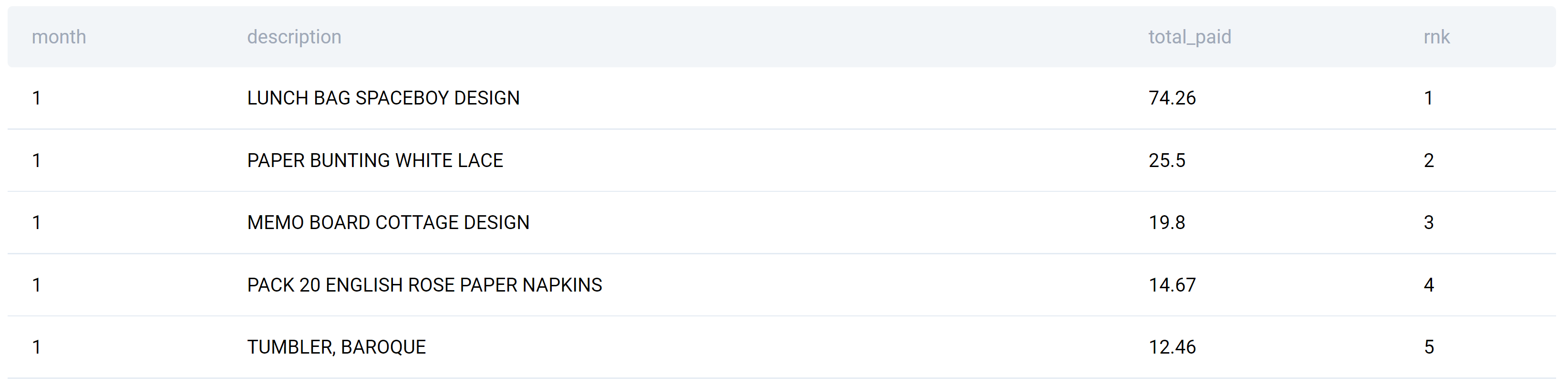
For you to easier comprehend what this query does, here’s its output.

6. Make the SELECT Statement a Subquery
Now, this query result has to be used in another SELECT statement. Therefore, we need to make it a subquery.
SELECT
FROM
  (SELECT DATE_PART('month', invoicedate) AS MONTH,
          description,
          SUM(unitprice * quantity) AS total_paid,
          RANK() OVER (PARTITION BY date_part('month', invoicedate)
                       ORDER BY SUM(unitprice * quantity) DESC) AS rnk
   FROM online_retail
   GROUP BY MONTH,
            description) AS rnk;
The subquery is named rnk and will be used by the main SELECT statement as a table in the FROM clause.
7. SELECT Required Data From a Subquery
The output has to show month, description, and the sales amount, so we have to select these columns in the main SELECT.
SELECT month,
       description,
       total_paid
FROM
  (SELECT DATE_PART('month', invoicedate) AS MONTH,
          description,
          SUM(unitprice * quantity) AS total_paid,
          RANK() OVER (PARTITION BY date_part('month', invoicedate)
                       ORDER BY SUM(unitprice * quantity) DESC) AS rnk
   FROM online_retail
   GROUP BY MONTH,
            description) AS rnk;
8. Use WHERE Clause to Show the Bestselling Product Each Month
Once you filter data, you get the question solution.
SELECT month,
description,
total_paid
FROM
(SELECT DATE_PART('month', invoicedate) AS MONTH,
description,
SUM(unitprice * quantity) AS total_paid,
RANK() OVER (PARTITION BY date_part('month', invoicedate)
ORDER BY SUM(unitprice * quantity) DESC) AS rnk
FROM online_retail
GROUP BY MONTH,
description) AS rnk
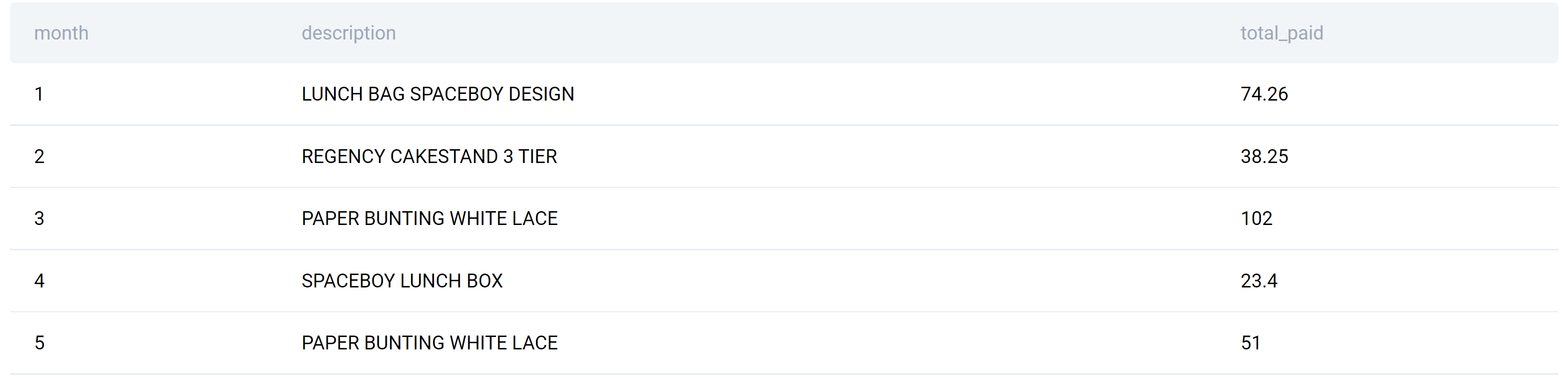
WHERE rnk = 1;
The solution gives the following output.

Question #3 Value Window Function: Year Over Year Churn
The value window functions offer you different possibilities to access values from other rows. The question by Lyft tests exactly that.

Link to the question: https://platform.stratascratch.com/coding/10017-year-over-year-churn
Solution Approach
1. Exploring the Dataset
The one table you’ll use here is lyft_drivers.
| index: | int |
| start_date: | datetime |
| end_date: | datetime |
| yearly_salary: | int |
This is a list of Lyft drivers. The only way to identify them is the column index, so it should be unique. The start_date should never be NULL, because the drivers can’t be in the list if they didn’t start working. However, the end date will probably have some NULL values: if it is NULL, the driver is still working for Lyft. Also, every driver has to have a salary.
We can confirm our assumptions by previewing the data.
You see that all index values are unique, and all the drivers have a start date and a salary. This preview shows that all the drivers from 0 to 5 are still there, while the driver number 6 has left on 6 August 2018.
2. Identifying Columns for Solving the Question
The question asks to show data on a yearly level, so we will need to use the column end_date. This is the only column we will have to explicitly use to get the solution.
3. Writing Out the Code Logic
This is how the code can be broken down.
- SELECT and DATE_PART() – to get the year from end_date
- WHERE clause – to show only drivers that left the company
- Subquery – write it as a subquery in the FROM clause
- SELECT year from the subquery
- COUNT(*) – to count the number of drivers that left the company in every year
- LAG() – to get the numbers of drivers that left the company the previous year
- GROUP BY – to show data on a yearly level
- ORDER BY – to sort data from the oldest to the newest year
- Subquery and SELECT all – write this as a subquery in the FROM clause, too, and select all columns from it
- CASE statement – to label the output columns as ‘increase’, ‘decrease’, and ‘no change’
4. Coding
1. SELECT & DATE_PART()
Use the the column end_date in the DATE_PART() function to output the year from the table lyft_drivers.
SELECT DATE_PART('year', end_date::date) AS year_driver_churned
FROM lyft_drivers;
Additionally, format years as date type.
2. WHERE Clause
We will use the WHERE clause to show only those drivers that left the company. From inspecting the available data, we know those are drivers that have the non-NULL values in the column end_date.
SELECT DATE_PART('year', end_date::date) AS year_driver_churned
FROM lyft_drivers
WHERE end_date IS NOT NULL;
Before we turn it into a subquery, let’s see what this part of code returns.

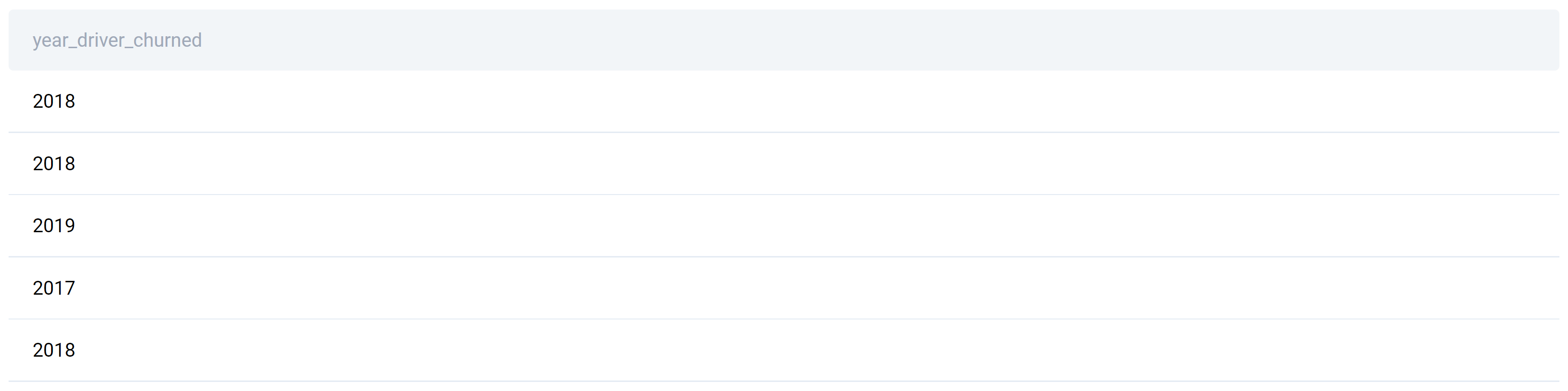
This is a list of years, with every year representing one driver that left. The years are duplicate because it’s possible that more than one drivers has left that year.
3. Write SELECT as a Subquery
This subquery has to appear in the FROM clause of the main query, so it can be used as a table. The subquery’s name is base.
SELECT
FROM
(SELECT DATE_PART('year', end_date::date) AS year_driver_churned
      FROM lyft_drivers
WHERE end_date IS NOT NULL) AS base;
4. SELECT Year From the Subquery
The column we need to select is year_driver_churned.
SELECT year_driver_churned
FROM
  (SELECT DATE_PART('year', end_date::date) AS year_driver_churned
   FROM lyft_drivers
   WHERE end_date IS NOT NULL) AS base;
5. Count the Number of Drivers That Left the Company
We will use the COUNT(*) function. It will count the number of rows, which equals the number of drivers.
SELECT year_driver_churned,
       COUNT(*) AS n_churned
FROM
  (SELECT DATE_PART('year', end_date::date) AS year_driver_churned
   FROM lyft_drivers
   WHERE end_date IS NOT NULL) AS base;
6. Use LAG() Window Function
Now comes the interesting part! The LAG() function allows you to access the data from the previous rows. We will use it to find the number of drivers that left the previous year.
SELECT year_driver_churned,
       COUNT(*) AS n_churned,
       LAG(COUNT(*), 1, '0') OVER (
                                   ORDER BY year_driver_churned) AS n_churned_prev
FROM
  (SELECT DATE_PART('year', end_date::date) AS year_driver_churned
   FROM lyft_drivers
   WHERE end_date IS NOT NULL) AS base;
The first argument in LAG() is the value we want to return, which is a number of drivers.
The integer 1 is the number of rows we want to go back in relation to the current row. In other words, going back one row means we’re going one year back.
The text value '0' specifies the value to be returned if there are no previous values. This will mean that when we show the first available year, the churn from the previous year will appear as zero. If this argument is left out, the default value will be NULL.
The data in the OVER() clause is sorted ascendingly by the year. By that, we are ordering data chronologically, so that the previous row will always mean previous year.
7. GROUP BY Year
This part of code will group together all drivers that left in the same year.
SELECT year_driver_churned,
       COUNT(*) AS n_churned,
       LAG(COUNT(*), 1, '0') OVER (
                                   ORDER BY year_driver_churned) AS n_churned_prev
FROM
  (SELECT DATE_PART('year', end_date::date) AS year_driver_churned
   FROM lyft_drivers
   WHERE end_date IS NOT NULL) base
GROUP BY year_driver_churned;
8. Use ORDER BY to Sort the Output Chronologically
The output is sorted by the column year_driver_churned.
SELECT year_driver_churned,
       COUNT(*) AS n_churned,
       LAG(COUNT(*), 1, '0') OVER (
                                   ORDER BY year_driver_churned) AS n_churned_prev
FROM
  (SELECT DATE_PART('year', end_date::date) AS year_driver_churned
   FROM lyft_drivers
   WHERE end_date IS NOT NULL) base
GROUP BY year_driver_churned
ORDER BY year_driver_churned ASC;
These two SELECT statements give this output.

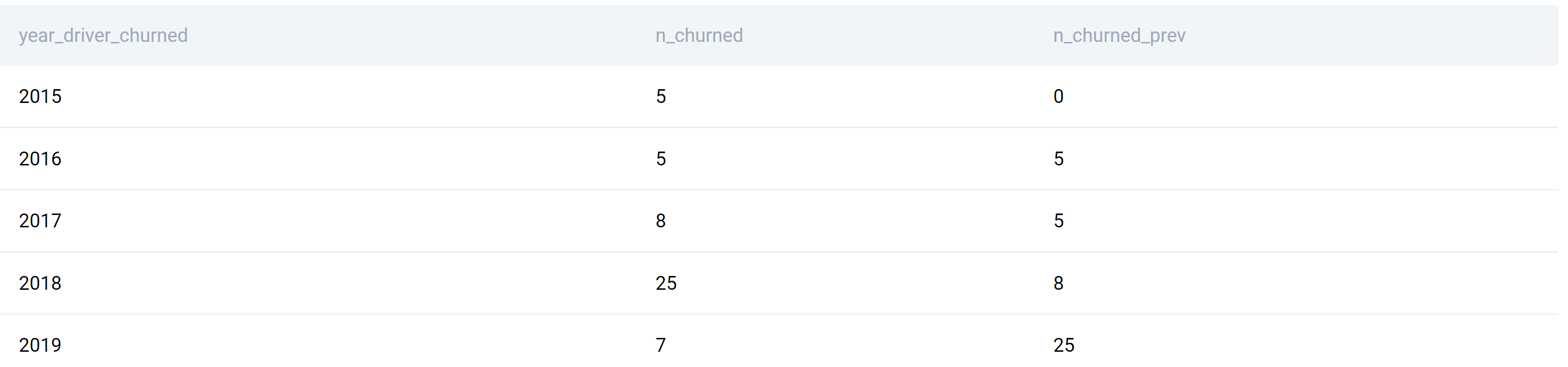
There’s data for years 2015 to 2019.
The data tells us 5 drivers churned in 2015, while no drivers churned in the previous year because there’s no data for 2014. In 2016, again 5 drivers churned, which is the same as in the previous year. The column n_churned_prev takes data from the previous year and shows it in the current year’s row.
9. Write the Second Subquery and Select All Data From It
Again, this second subquery appears in the FROM clause.
SELECT *
FROM
  (SELECT year_driver_churned,
          COUNT(*) AS n_churned,
          LAG(COUNT(*), 1, '0') OVER (
                                      ORDER BY year_driver_churned) AS n_churned_prev
   FROM
     (SELECT DATE_PART('year', end_date::date) AS year_driver_churned
      FROM lyft_drivers
      WHERE end_date IS NOT NULL) base
   GROUP BY year_driver_churned
   ORDER BY year_driver_churned ASC) AS calc;
10. Label Data Using CASE
The CASE statement will label the output data. If the churned number is higher than in the previous year, this will mean an increase. If it’s lower, the label will be ‘decrease’. When it’s neither, it well be marked as no change.
By writing the CASE statement you’ve completed answering this SQL window functions interview question.
SELECT *,
       CASE
           WHEN n_churned > n_churned_prev THEN 'increase'
           WHEN n_churned < n_churned_prev THEN 'decrease'
           ELSE 'no change'
       END
FROM
  (SELECT year_driver_churned,
          COUNT(*) AS n_churned,
          LAG(COUNT(*), 1, '0') OVER (
                                      ORDER BY year_driver_churned) AS n_churned_prev
   FROM
     (SELECT DATE_PART('year', end_date::date) AS year_driver_churned
      FROM lyft_drivers
      WHERE end_date IS NOT NULL) base
   GROUP BY year_driver_churned
   ORDER BY year_driver_churned ASC) AS calc;
As for output, here it is.

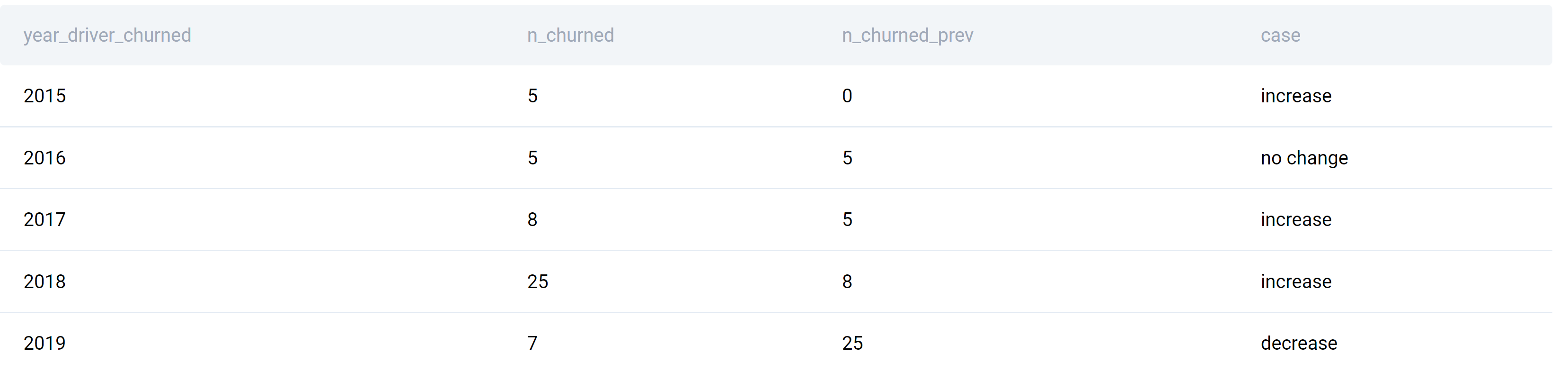
It’s the same as the one we showed earlier, except this one is labeled.
Summary
Hopefully these three examples show you the power of the SQL window functions. They are necessary for anyone doing even remotely useful data analysis in SQL.
Of course, you can expect the window functions to come up at the job interview. Because of that, you should dedicate some time to practicing. If you want to make your interview preparation as efficient as possible, take a look at our selection of SQL Query Interview Questions curated according to the most popular SQL concepts tested in interviews.
Share