Machine Learning Algorithms Explained: Anomaly Detection


 Written by:
Nathan Rosidi
What is anomaly detection in machine learning? This in-depth article will give you an answer by explaining how it is used, its types, and its algorithms.
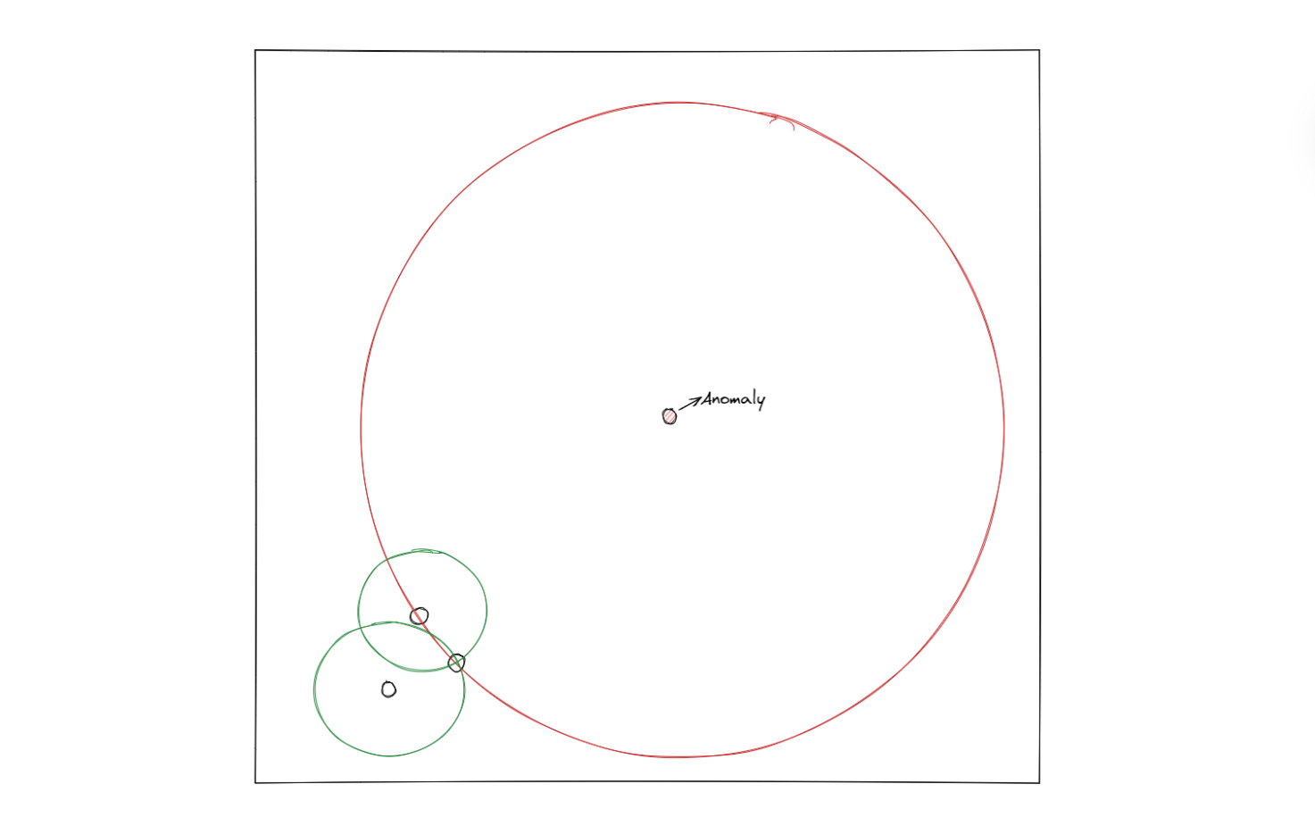
In this article, we are going to talk about anomaly detection, which is one of many applications within machine learning applications. To understand intuitively what anomaly detection in machine learning is, let’s take a look at the following illustration of six arbitrarily chosen objects:

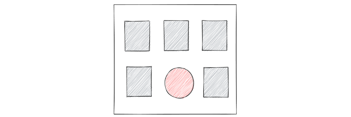
Which one do you think is the odd one out of the six objects above? If you’re choosing the red circle, then congratulations, you just did an anomaly detection! Anomaly detection in machine learning refers to the process of identifying unusual patterns from the data.
Humans normally can do a great job in identifying unusual patterns in data, as long as the data is small and there is no time constraint. However, as the data gets bigger, then it becomes impossible for humans to perform anomaly detection in a quick manner, and we definitely need something that can automate this process for us. This is where we need machine learning to perform anomaly detection.
Nowadays, machine learning algorithm for anomaly detection has been implemented in a lot of areas within real-world applications, for example:
- In the financial sector: machine learning algorithms have been implemented to detect suspicious and fraudulent transaction activity so that preventive measures can be taken into account
- In the health sector: anomaly detection algorithms have been implemented to assist doctors in making more accurate diagnoses by detecting unusual patterns in the MRI scan results.
- In the infrastructure sector: anomaly detection algorithms have been implemented in various infrastructures, such as railway systems, where the detection of potential damage would be very crucial for the safety of the passengers.
As you can see, anomaly detection is such an important method in machine learning due to the wide variety of real-life use cases. In this article, we’re going to look at several anomaly detection algorithms commonly used in real life, such as:
- Gaussian Mixture Model
- Kernel Density Estimation
- Isolation Forest
- Local Outlier Factor
- DBSCAN
- One-Class SVM
Approach for Anomaly Detection in Machine Learning

Before we dig deeper into each anomaly detection algorithm, let’s talk about the general surface-level approach behind the training process of any anomaly detection algorithm. In general, there are three different approaches to train an anomaly detection algorithm: supervised, unsupervised, and semi-supervised.
- Supervised: this approach requires human intervention in the sense that we need to provide the algorithm with a label for each data before the training process. The label normally consists of two possible values, e.g., normal data points will be labeled as 1, and anomalous data points will be labeled as 0 or -1.
- Unsupervised: this approach doesn’t require human intervention because we don’t need to provide the ground truth label of each data point to the algorithm before the training process. In other words, the algorithm will learn the pattern of the data points during the training process by itself. Then, based on the density of each data point, the algorithm will decide whether a data point is an outlier or not.
- Semi-supervised: this approach is a combination of the previous two approaches. This means that only small portions of the data are labeled. This technique is useful in real life because it is nearly impossible to provide the label of each data point given the huge size of real-life data.
Now that we know different approaches to training anomaly detection algorithms, let’s start to delve deeper into each of the common anomaly detection algorithms, starting from the Gaussian Mixture Model.
Gaussian Mixture Model
If you’ve read this article about supervised vs unsupervised learning, you’ll probably know that we normally use the Gaussian Mixture Model (GMM) for clustering purposes. However, we can use GMM for anomaly detection too.
GMM is a probability-based method that assumes that a data point in our datasets comes from a particular Gaussian distribution. What we normally do with GMM is the following:
- First, we need to define the total number of Gaussian distributions in advance. Thus, this is a hyperparameter that we should fine-tune in order to get the optimal result. We will see how we can come up with the optimal number of Gaussian distributions in the next section.
- The parameters (mean and standard deviation) of each Gaussian distribution that we initialized in the first step will be initialized randomly.
- Next, with an iterative approach, the parameters of each Gaussian distribution will be optimized such that in the end, each distribution will represent the most likely distribution of a cluster of data points.
The iterative approach of a GMM method consists of two steps: an expectation step and a maximization step.
- In the expectation step, each data point will be assigned to a random Gaussian distribution. The purpose of this step is basically to answer: does the assigned data point have a high likelihood of being generated from that particular Gaussian distribution?
- In the maximization step, each of the Gaussian distribution’s parameters (mean, standard deviation, and weight) will be updated according to the likelihood of each data point being generated from that Gaussian distribution.
In a nutshell, the concept of GMM for anomaly detection in machine learning is really simple. Let’s say we have data points scattered in 2-dimensional space. If a data point is located in a high-density region of the optimized Gaussian distribution, then we consider those data points as normal. Meanwhile, if a data point is located in a low-density region, then that particular data point will be classified as an outlier.
With GMM, it is necessary for us to set up a threshold value for the proportion of outliers in our dataset in advance. So let’s say that based on our judgment and knowledge about the data, we decide that a data point can be considered as an outlier if it’s located in the area below the 10% percentile, then we can specify that in advance. We will see an example of how to do this in the implementation section.
Implementation of Gaussian Mixture Model
In this section, we will implement the GMM algorithm for anomaly detection with the help of scikit learn algorithm. But first, let’s generate the dataset that we will use for all of the examples in this article. We will create a blobs dataset consisting of 120 data points.
import numpy as np
import matplotlib.pyplot as plt
from sklearn.datasets import make_blobs


X, y_true = make_blobs(n_samples=100, centers=1, cluster_std=0.8, random_state=5)

X_append, y_true_append = make_blobs(n_samples=20,centers=1, cluster_std=5,random_state=5)

X = np.vstack([X,X_append])
y_true = np.hstack([y_true, [1 for _ in y_true_append]])


plt.figure(figsize=(12,9))
X = X[:, ::-1]
plt.grid(True)
plt.scatter(X[:,0],X[:,1],marker="s");
And this is the visualization of our data points that you’ll get after executing the code snippet above.


Now we are ready to implement the GMM algorithm. Let’s say that we have decided that data points that are located below the 10% percentile of a cluster can be considered as outliers. To do this, first, we need to train our GMM model on our datasets.
gmm = GaussianMixture(n_components=1)
gmm.fit(X)
After we train our GMM model, we can fetch the log-likelihood score of each data point by using the score_samples() method. We can use this score to detect anomalous data points.
scores = gmm.score_samples(X)
print(scores[0:5])

# [-3.54611177 -3.22356918 -3.25026183 -3.24526915 -3.3393749 ]
Now let’s try to compute the threshold value that we should define to decide whether a data point is an anomaly or not. As mentioned previously, we assume that the data points that are located below 10% of a cluster can be classified as an anomaly. To transform this logic into a threshold value, we can use quantile() method from numpy.
thresh = quantile(scores, 0.1)
print(thresh)

# -5.623547106080151
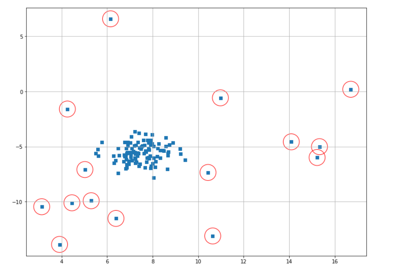
This means that if a log-likelihood value of a data point is smaller than -5.6, then that data point can be considered as an anomaly. Finally, we can fetch the index of data points that have a log-likelihood value smaller than the threshold and then plot the result.
index = where(scores <= thresh)
# Circling of anomalies
plt.figure(figsize=(12,9))
plt.grid(True)
plt.scatter(X[:,0],X[:,1],marker="s");
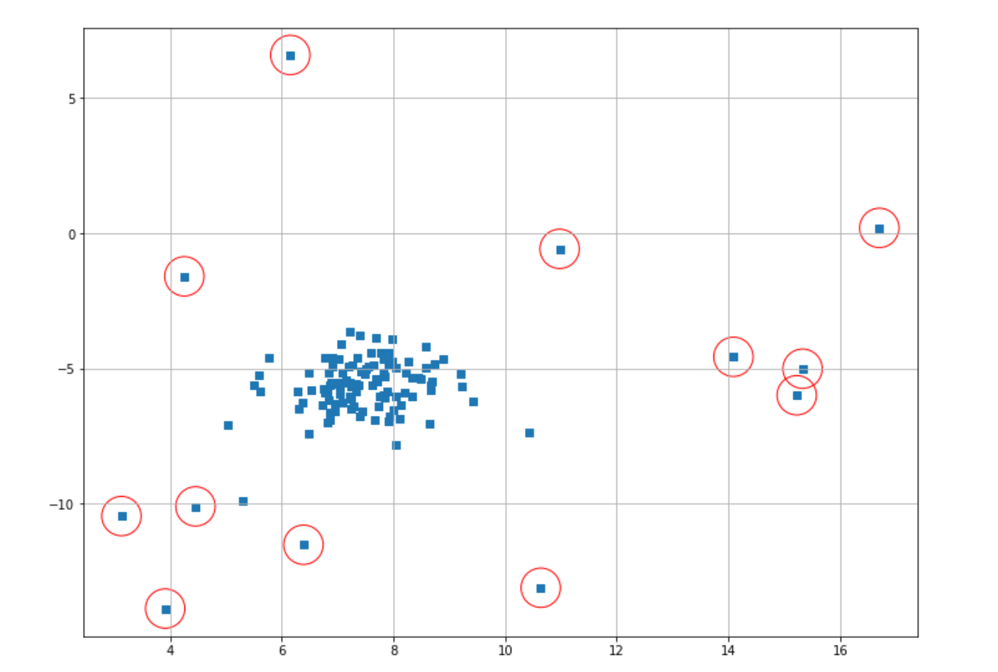
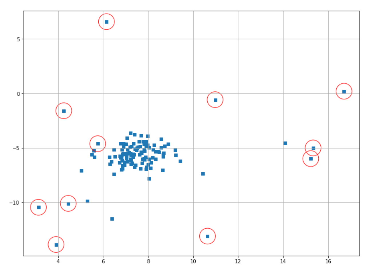
plt.scatter(X[index,0],X[index,1],marker="o",facecolor="none",edgecolor="r",s=1000);
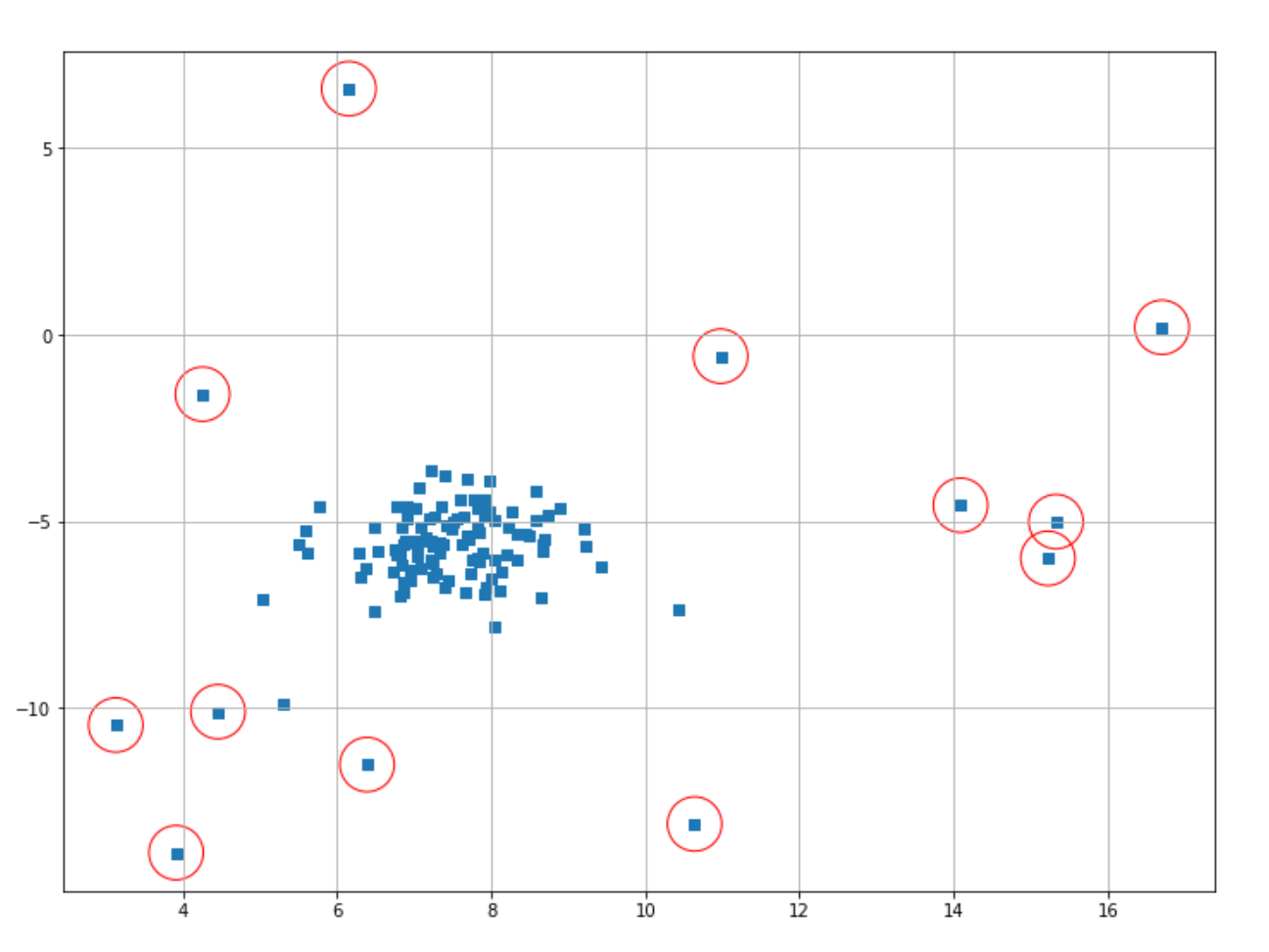
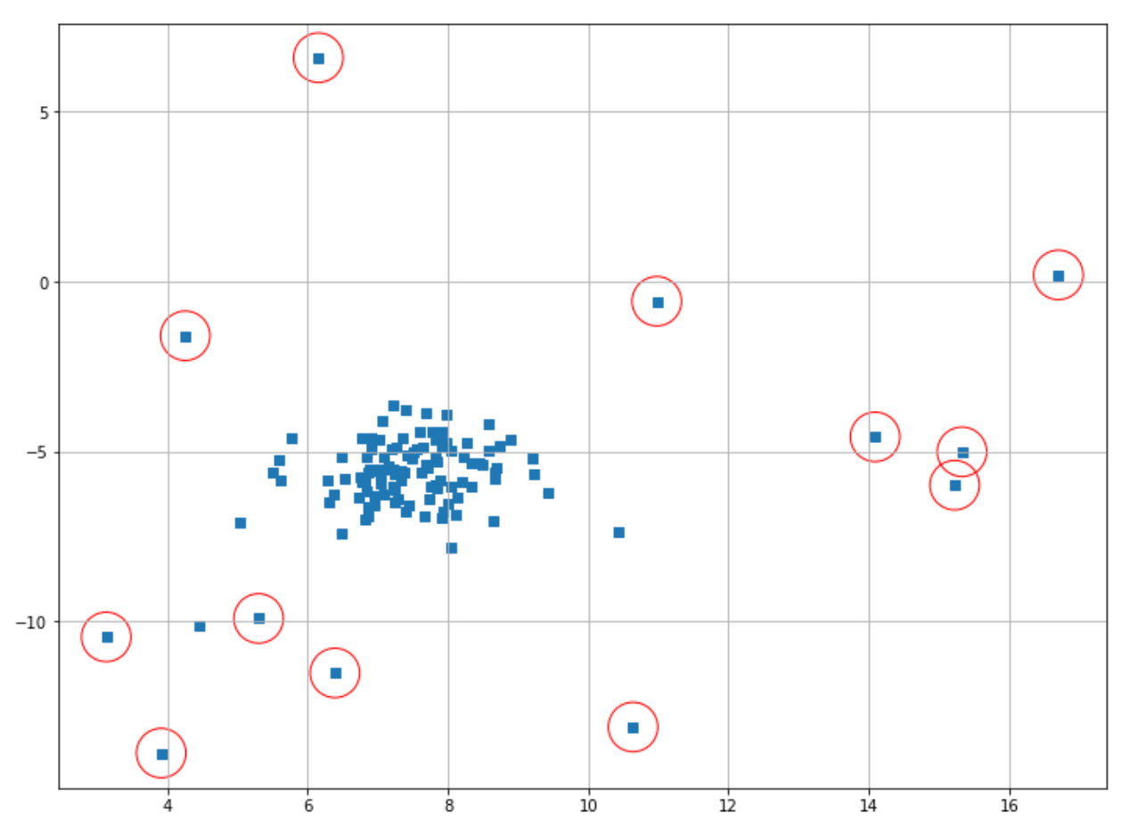
The data points classified as anomalies are shown in red circles. It’s important to note that it’s still us who need to decide the threshold value for a data point to be classified as an anomaly.
Thus, if we feel like there are too many false positive results (i.e too many ‘normal’ data points are being classified as an anomaly), then we can decrease the threshold value. Likewise, if we feel that there are too many false negatives (i.e too many anomalies are being classified as ‘normal’ data points), then we can increase the threshold value.
Kernel Density Estimation
Kernel Density Estimation or commonly abbreviated as KDE is an unsupervised learning algorithm that can also be useful for anomaly detection in machine learning. If you know the concept of a histogram, then it will be easy to understand the concept of KDE.
As you might already know, a histogram visualizes data points into bins, where each bin corresponds to the total number of data points it represents, as you can see in the following visualization:

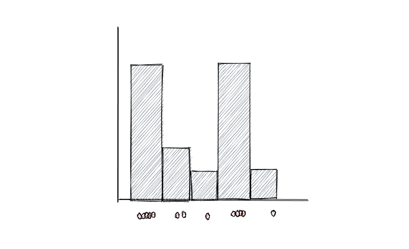
One major disadvantage of using bins to represent data points is that if we change the size of each bin, then the resulting histogram will be affected, which then might lead to the wrong interpretation of data. For anomaly detection purposes, a KDE algorithm usually uses Gaussian distribution to replace the bins in the histogram to smoothen the distribution of data points. As a result, a smooth density estimate can be derived from our data, as you can see in the visualization below:

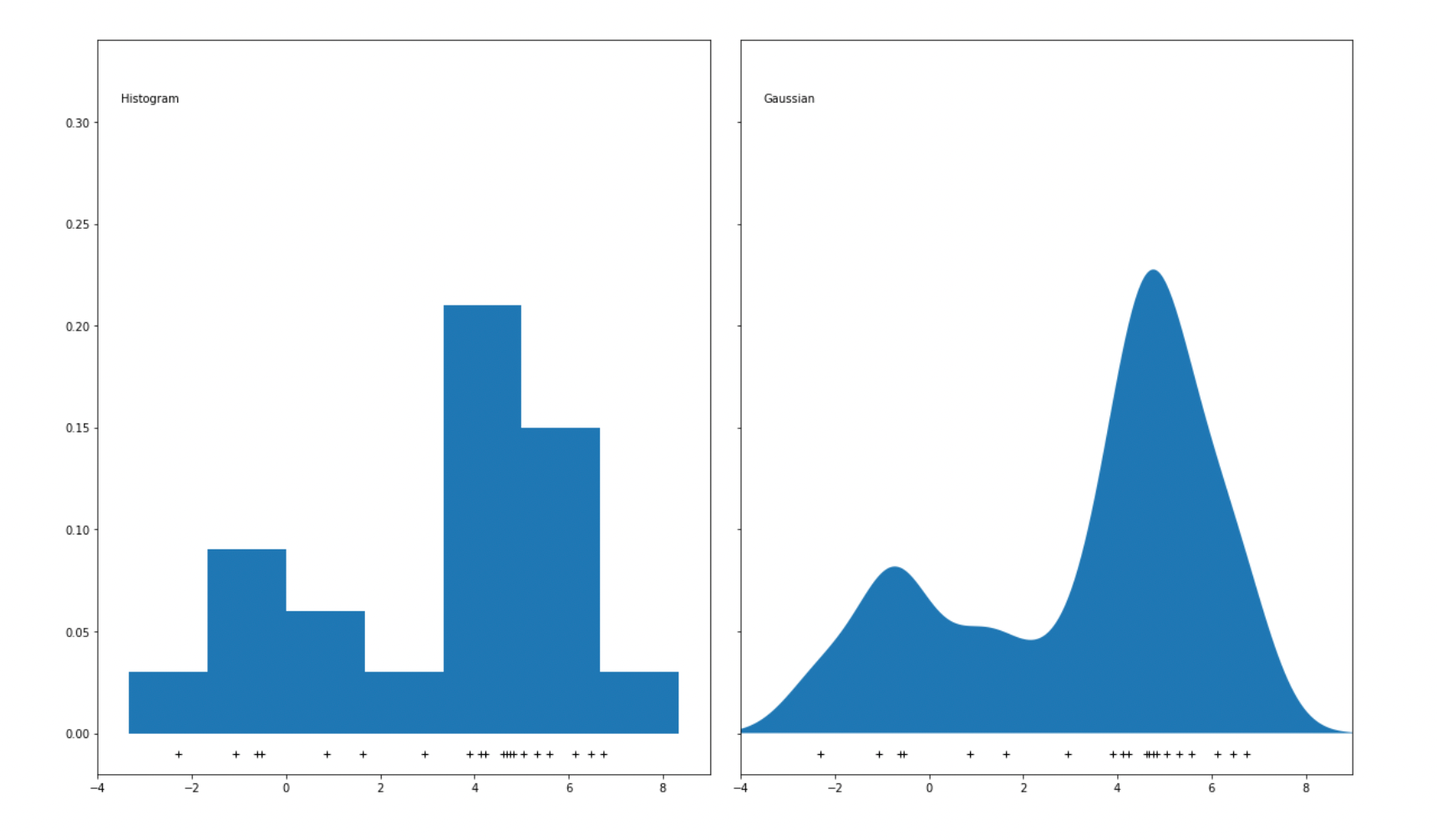
Gaussian distribution is not the only estimator that we can use to apply the KDE algorithm, as we can use some other estimators such as tophat, exponential, linear, cosine, or epanechnikov, as you can see in the visualization below:

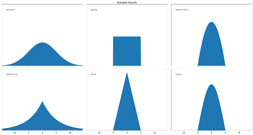
So with these various estimators, how can we find out whether a data point is an anomaly or not? Given the estimator of our choice, the density of a data point y within the group of data points xi can be calculated with the following equation:
where:
ρ: density
N: total number of data points
h: a bandwidth parameter, the larger the bandwidth, the smoother the distribution will be.
K: estimator
The equation of K depends on the estimator that we use. In the case of Gaussian, then the equation would be:
If the resulting density of a point y is below a threshold value that we define in advance, then that data point can be considered an anomaly. Likewise, if a data point has a density that is above the threshold value, then we can say that the data point is a normal data point.
Implementation of Kernel Density Estimation
Implementing KDE with Python can be easily done with the help of the scikit-learn library. To instantiate a KDE model with a Gaussian estimator, we can use KernelDensity class from sklearn.neighbors. Next, we can train our model on our dataset.
from sklearn.neighbors import KernelDensity

density_est = KernelDensity().fit(X)
Same as GMM in the previous section, after we trained our KDE model, we can fetch the log-likelihood score of each data point with the score_samples method, as you can see below:
scores_de = density_est.score_samples(X)
print(scores_de[0:5])

# [-3.4430811  -2.60158452 -2.69253285 -2.74078121 -2.82694107]
Next, we also need to define the threshold value with the same approach shown in the GMM section above. Let’s say that we assume that data points that are located below 10% of a cluster should be classified as anomalies, then we can define the threshold value for that with the quantile method.
thresh = quantile(scores_de, 0.1)
print(thresh)

# -5.866011376650252
Next, we can fetch the index of data points that will be classified as anomalies based on the threshold value and then visualize the result.
index = where(scores_de <= thresh)
# Circling of anomalies
plt.figure(figsize=(12,9))
plt.grid(True)
plt.scatter(X[:,0],X[:,1],marker="s");
plt.scatter(X[index,0],X[index,1],marker="o",facecolor="none",edgecolor="r",s=1000);
Isolation Forest
Just by looking at its name, you might have guessed that this algorithm utilizes tree-based methods to perform anomaly detection in machine learning, and that’s absolutely the case. Since this is a tree-based algorithm, then the decision logic behind Isolation Forest is very similar to the Random Forest algorithm, which we normally use to solve regression or classification problems.

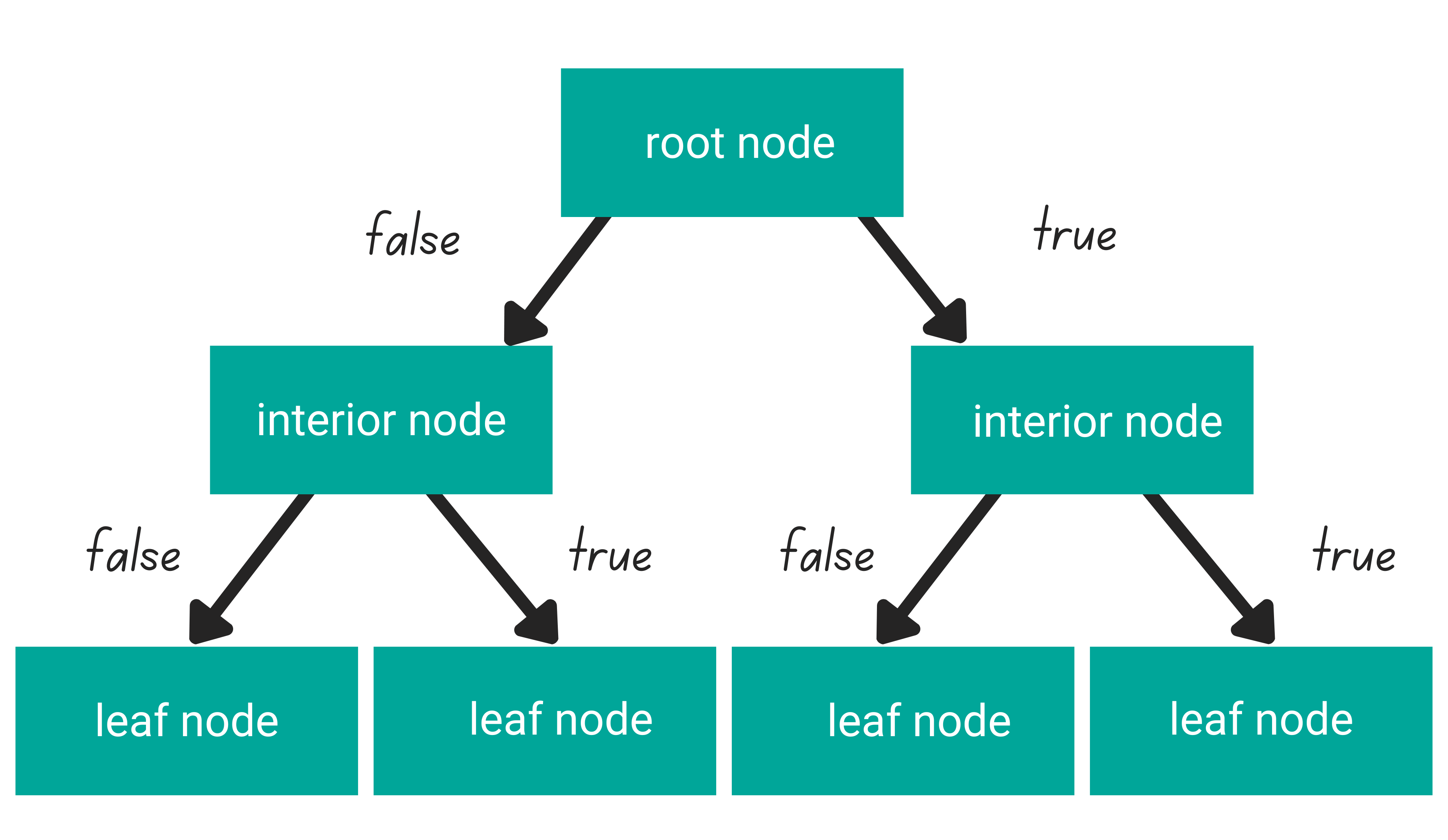
In general, tree-based algorithms have three different parts: one root node, several interior nodes, and several leaf nodes.
- A root node is the purest feature in our dataset
- Several interior nodes consist of the rest of the features in our dataset
- Several leaf nodes consist of the prediction of our tree-based algorithm
The logic that connects one level of a node to another is called a branch. In each level of the node, each data point’s value will be checked to decide in which branch it should go: whether to the left branch or to the right branch. This process will be repeated at each level of the node until the data point reaches the leaf node.
You can learn more about tree-based algorithm via this article “Decision Tree and Random Forest Algorithm Explained”.
Isolation forest is a tree-based anomaly detection algorithm, and it has a similar structure to the illustration that you can see above. The logic behind the isolation forest algorithm is that data points that are considered anomalies would be closer to the root of the tree compared to normal data points.
Let’s use an example to make this point even more clear.
Suppose that we’re collecting data about people’s net worth, and one of the samples happened to be Elon Musk. We know that Elon Musk’s net worth is beyond normal people's net worth. Thus, when we use Isolation Forest, the name Elon Musk would appear close to the root node compared to normal people, as you can see in the following illustration:


A data point that can be considered as an anomaly has a very distinguishable value in comparison with other data points and often provides a pure separation of a feature in our dataset, which makes it easy for tree-based algorithms to split this data point. Now to decide whether a data point can be considered as an outlier, the Isolation Forest algorithm uses the following equation:
where:
In the above equation:
s(x,n): anomaly score which has a value between 0 to 1, the higher the value, the more likely that a data point is an anomaly.
n: number of data points
h(x): the depth of the tree in which a data point is found
H: a harmonic number, where H(i) can be estimated by ln(i) + 0.577
E(h(x)): average of h(x) across different trees
As you can see from the equation above, the variable h represents the depth of the tree to which data point is found. The closer a data point to the root node, the smaller its depth would be, and if we compute the equation above, the smaller the h, the higher the resulting s, which represents the anomaly score. The higher the anomaly score, the more likely it is that a data point is an outlier.
Implementation of Isolation Forest Algorithm
In this section, we’re going to implement the Isolation Forest algorithm with the help of the scikit-learn library. In the code snippet below, first, we instantiate our model from sklearn.ensemble and then train the model with our data.
from sklearn.ensemble import IsolationForest

iso_forest =IsolationForest()
prediction = iso_forest.fit_predict(X)
With the fit_predict method, we basically trained our model on our data, and after that, it will return the label of each data point. With Isolation Forest, what we will get from the fit_predict method is a binary value: it’s either 1 or -1. As you might have guessed, if a data point is labeled as -1, then that data point can be considered as an anomaly, and vice versa, if a data point is labeled as 1, then we can say that particular data point is a normal one.
Now, let’s mark data points that have been labeled as outliers with a red circle. Then, we can visualize the result straight away.
index = where(prediction == -1)
# Circling of anomalies
plt.figure(figsize=(12,9))
plt.grid(True)
plt.scatter(X[:,0],X[:,1],marker="s");
plt.scatter(X[index,0],X[index,1],marker="o",facecolor="none",edgecolor="r",s=1000);
Local Outlier Factor (LOF)
If you are already familiar with how the k-Nearest Neighbors algorithm works, then you’ll understand how Local Outlier Factor (LOF) works. LOF is an algorithm commonly used for outlier detection that utilizes the same concept as k-Nearest Neighbors, as it uses the distance to a particular number of neighbors as one of the criteria whether a data point can be considered as an outlier or not.
If we take a brief look at how the k-Nearest Neighbors algorithm works, we need to define the number of neighbors in advance. Let’s say that we pick the number of neighbors equal to 4. When we have an unseen data point, the four nearest neighbors of that data point will be computed and the majority label of its four neighbors will determine its label.
The concept of LOF is similar. First, we need to define the number of neighbors in advance. Then the distance between each data point in our dataset to each of its neighbors will be computed. The distance between each data point and its neighbor is called reachability distance. We can compute the reachability distance with the following equation:
Now that we know the concept of reachability distance, the next concept that we should know is the local reachability distance. The local reachability distance can be described as the inverse of the average reachability. Mathematically, we can compute the local reachability distance with the following equation:
What LOF does is that it compares the average local reachability distance of a data point to its nearest neighbors with the local reachability distance of that data point itself.

From the equation above, then in the end we will get the final LOF value. The common rule of thumb is that if the resulting LOF value is greater than one, then we can consider a particular data point as an anomaly. This is because the value greater than one indicates that the distance between a data point to its neighbors is longer than the distance between each neighbor to the other neighbors.
Implementation of Local Outlier Factor
Now that we know the theory of LOF, let’s implement it with Python. To do this, we can use the scikit-learn library and instantiate our model from sklearn.neighbors method. Next, we can train our model on our data, as you can see in the code snippet below:
from sklearn.neighbors import LocalOutlierFactor

lof = LocalOutlierFactor(novelty=True)
lof.fit(X)
In the above method, we need to set the parameter novelty to True in order for us to be able to calculate the LOF equation that we have seen in the theory above with score_samples method, as you can see below:
score_lof = lof.score_samples(X)
print(score_lof[0:5])

# [-1.29347918 -0.98582756 -1.01736912 -1.05872722 -1.06295241]
One important thing to note is that the result that we got from score_samples method above is the opposite of the LOF equation that we have seen in the previous section. With the original LOF equation, the bigger the value that we get, the more likely it is that a data point is an anomaly. Meanwhile, the result that we get from score_samples above is the opposite of that, which means that the smaller the value that we get, the more likely it is that a data point is an anomaly.
Now that we have the LOF value for each data point, we can set the threshold value with the same approach as the previous algorithms. Let’s say that we set that 10% of our data points are anomalous, then we can find our threshold value as follows:
thresh = quantile(score_lof, 0.1)
print(thresh)
# -3.63597749802095
Finally, we can mark the anomalous data points with red circles and visualize the result.
index = where(score_lof <= thresh)
# Circling of anomalies
plt.figure(figsize=(12,9))
plt.grid(True)
plt.scatter(X[:,0],X[:,1],marker="s");
plt.scatter(X[index,0],X[index,1],marker="o",facecolor="none",edgecolor="r",s=1000);

With LOF, there is one important hyperparameter that we can tune, which is the number of neighbors. If we don’t define it in advance, the number of neighbors will be set to 20 as the default value.
DBSCAN
Density Based Spatial Clustering of Applications with Noise or commonly abbreviated as DBSCAN is an unsupervised machine learning method that is commonly used for clustering purposes. However, it turns out that we can use it as well for anomaly detection in machine learning.
As the name suggests, this algorithm works by calculating the density of the neighborhood around a particular data point. If a data point is located in a dense neighborhood, then we can say that this point is a normal point and otherwise, an anomaly.
The DBSCAN algorithm calculates the density around the neighborhood of a data point by calculating the distance between data points. Specifically, below is the step-by-step explanation of how this algorithm works:
- Before we train a DBSCAN model, there are two hyperparameters that we should define in advance: the threshold distance and the minimum number of neighbors of a data point.
- Now, for each data point in our dataset, the neighbors that satisfy the threshold distance will be counted.
- If the number of neighbors of a data point fulfills the minimum number of neighbors that we have defined in advance, then that data point will become the so-called core sample. A core sample is a data point that is located in a region with high density.
- The neighbors of a core sample will then be grouped together into one cluster
- If any of the data points is not a neighbor of any core sample, then that data point will be considered as an anomaly
Implementation of the DBSCAN Algorithm
Same as our previous examples, we can implement DBSCAN with Python easily with the help of the scikit-learn library. First, let’s instantiate our model with the default value of threshold distance (epsilon), which is 0.5, and the default value of the minimum number of neighbors (min_samples), which is 5. Next, we will fit our DBSCAN model to our data.
from sklearn.cluster import DBSCAN

dbscan_model = DBSCAN()
dbscan_model.fit(X)
Now that we trained our model, we can fetch the label of each data point with the label_ method. This method will return the cluster to which each data point belongs. If a data point doesn’t belong to any cluster, it will be labeled as -1, which also means that this particular data point is an outlier.
Now we can find the index of the data points classified as an anomaly with a simple where method from numpy.
dbscan_label = dbscan_model.labels_
index = where(dbscan_label == -1)
Now we can mark anomalous data points with red circles and then visualize the result.

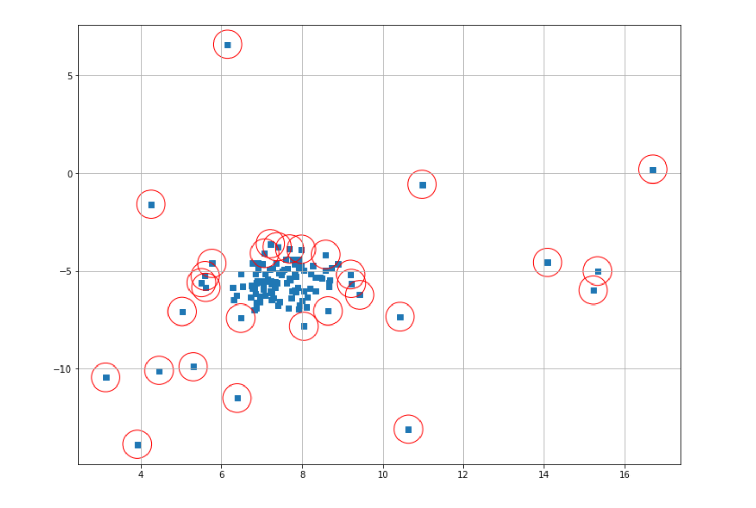
Now you might find that the result of our anomaly detection is not that good. This occurs due to the fact that we used the default value of epsilon when we instantiated our model in the beginning. In most cases, we should adjust the value of this hyperparameter in advance before we fit our model to our data. The problem is, in most cases, we don’t know the optimal value for epsilon.
However, there is a method that we can use in order to find the best epsilon value according to our data, and that is by visualizing the so-called k-distance graph. This graph visualizes the relationship between data points sorted by the distance and threshold distance value itself. To obtain this graph, first, we need to train a k-nearest neighbors model to our data, and then compute the distance between each data point to its closest neighbor, as you can see in the following code snippet:
from sklearn.neighbors import NearestNeighbors
neigh = NearestNeighbors(n_neighbors=2)
nbrs = neigh.fit(X)
distances, indices = nbrs.kneighbors(X)
Next, let’s sort the distance from closest to farthest, and then plot the k-distance graph as shown below:
# Plotting K-distance Graph
distances = np.sort(distances, axis=0)
distances = distances[:,1]
plt.figure(figsize=(20,10))
plt.plot(distances)
plt.xcorr
plt.title('K-distance Graph',fontsize=20)
plt.xlabel('Data Points sorted by distance',fontsize=14)
plt.ylabel('Epsilon',fontsize=14)
plt.show()
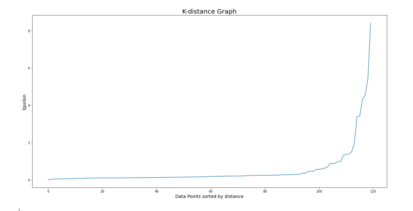
The optimal epsilon value would be the location in the graph where the elbow shape is formed, which in our visualization above can be approximated at epsilon = 1. So, let’s re-initialize our model and retrain our model, this time with epsilon value=1.
from sklearn.cluster import DBSCAN

dbscan_model = DBSCAN(eps=1)
dbscan_model.fit(X)
dbscan_label = dbscan_model.labels_
index = where(dbscan_label == -1)
# Circling of anomalies
plt.figure(figsize=(12,9))
plt.grid(True)
plt.scatter(X[:,0],X[:,1],marker="s");
plt.scatter(X[index,0],X[index,1],marker="o",facecolor="none",edgecolor="r",s=1000);
And now we’ve got a better result in our anomaly detection result. As you can see in the example above, the value of threshold distance is very important for us to get a good anomaly detection result. To get the optimal value of threshold distance, you can take a look at the k-distance graph of your data with the help of the k-nearest neighbors algorithm.
One-Class SVM
As the name suggests, One-Class SVM is an algorithm based on the Support Vector Machine (SVM) algorithm, which is one of the supervised machine learning algorithms commonly used for classification or regression purposes.
In a nutshell, an SVM algorithm tries to find the optimal boundary decision to separate data points into different classes by creating a so-called hyperplane with two margin lines. Let’s try to understand this concept better with an illustration.

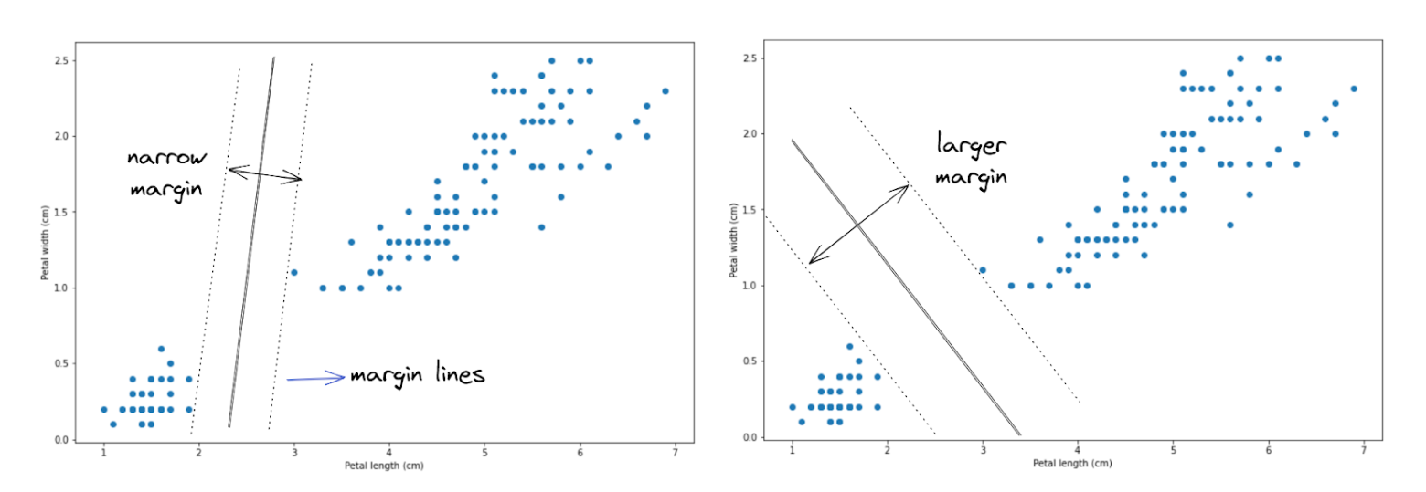
Let’s say that we have data points, as you can see above. To separate the data points into two different classes, there are a lot of possibilities of how a hyperplane can be created, and two out of those many possibilities are shown in the image above.
Two hyperplanes illustrated above seem to do a great job in separating data points into two classes, but which hyperplane does a better job? If you take a look, the hyperplane on the right-hand side does a better job because it allows the hyperplane to have wider margin lines compared to the hyperplane on the left-hand side. Thus, in the end, our SVM algorithm will create a hyperplane just like the image on the right-hand side to separate data points.
The illustration above shows how an SVM algorithm classifies two classes. With one-class SVM, the algorithm tries to classify data that consists of only one class, meaning that the hyperplane will have a spherical shape with a certain radius that needs to be minimized with an optimization procedure under the hood.

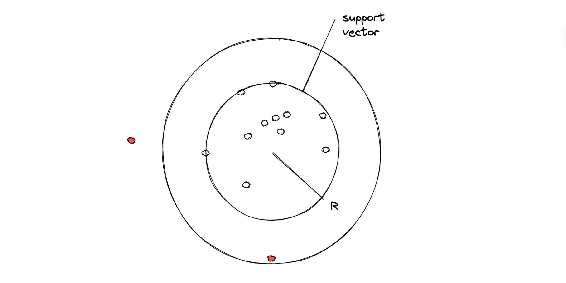
In the end, if a data point is inside the circle, then it will be considered an inlier, and vice versa, if a data point is outside of the circle, then it will be considered an outlier.
There is one hyperparameter that we can fine-tune in order to control the trade-off between the radius of the sphere and the number of data points that it can hold, which is the so-called nu (or ⋎) value. This ⋎ can take any value within the range of 0 to 1. The smaller the ⋎ value, we basically try to fit in more data points within the resulting sphere.
Implementation of One-Class SVM Algorithm
To implement One-Class SVM, we can also use the scikit-learn library, especially from sklearn.svm. As a first trial, let’s try to implement One-Class SVM with the default parameters from scikit-learn and see the result on our data points. First, let’s instantiate the model and then fit predict the data points with it.
from sklearn.svm import OneClassSVM

one_svm = OneClassSVM()
one_svm_label = one_svm.fit_predict(X)
Now that we have implemented the fit_predict function, we basically get the label of each data point that consists of two possible values, either 1 or -1. If a data point is considered as an outlier, then it will be labeled as -1. Let’s fetch the index of data points that have been labeled as outliers and then visualize the result.
index = where(one_svm_label == -1)
# Circling of anomalies
plt.figure(figsize=(12,9))
plt.grid(True)
plt.scatter(X[:,0],X[:,1],marker="s");
plt.scatter(X[index,0],X[index,1],marker="o",facecolor="none",edgecolor="r",s=1000);
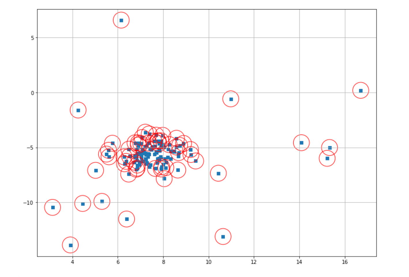
As you can see, our One-Class SVM performed poorly on our data points. But what might be the reason for this? As you might notice, in the first trial above, we implemented the One-Class SVM algorithm with the default parameter from scikit-learn. By default, the scikit-learn library uses 0.5 as the ⋎ value for our One-Class SVM algorithm.
As mentioned in the previous section, this hyperparameter determines the number of data points that try to be fitted inside the sphere. The larger the value, the fewer data points inside the sphere. The ⋎ value of 0.5 simply results in too many data points classified as outliers in our case. Thus, let’s reduce this value from 0.5 to 0.1 and then retrain our model.
from sklearn.svm import OneClassSVM

one_svm = OneClassSVM(nu=0.1)
one_svm_label = one_svm.fit_predict(X)
Now, let’s fetch the index of data points that are classified as outliers and then visualize the result.
index = where(one_svm_label == -1)
# Circling of anomalies
plt.figure(figsize=(12,9))
plt.grid(True)
plt.scatter(X[:,0],X[:,1],marker="s");
plt.scatter(X[index,0],X[index,1],marker="o",facecolor="none",edgecolor="r",s=1000);

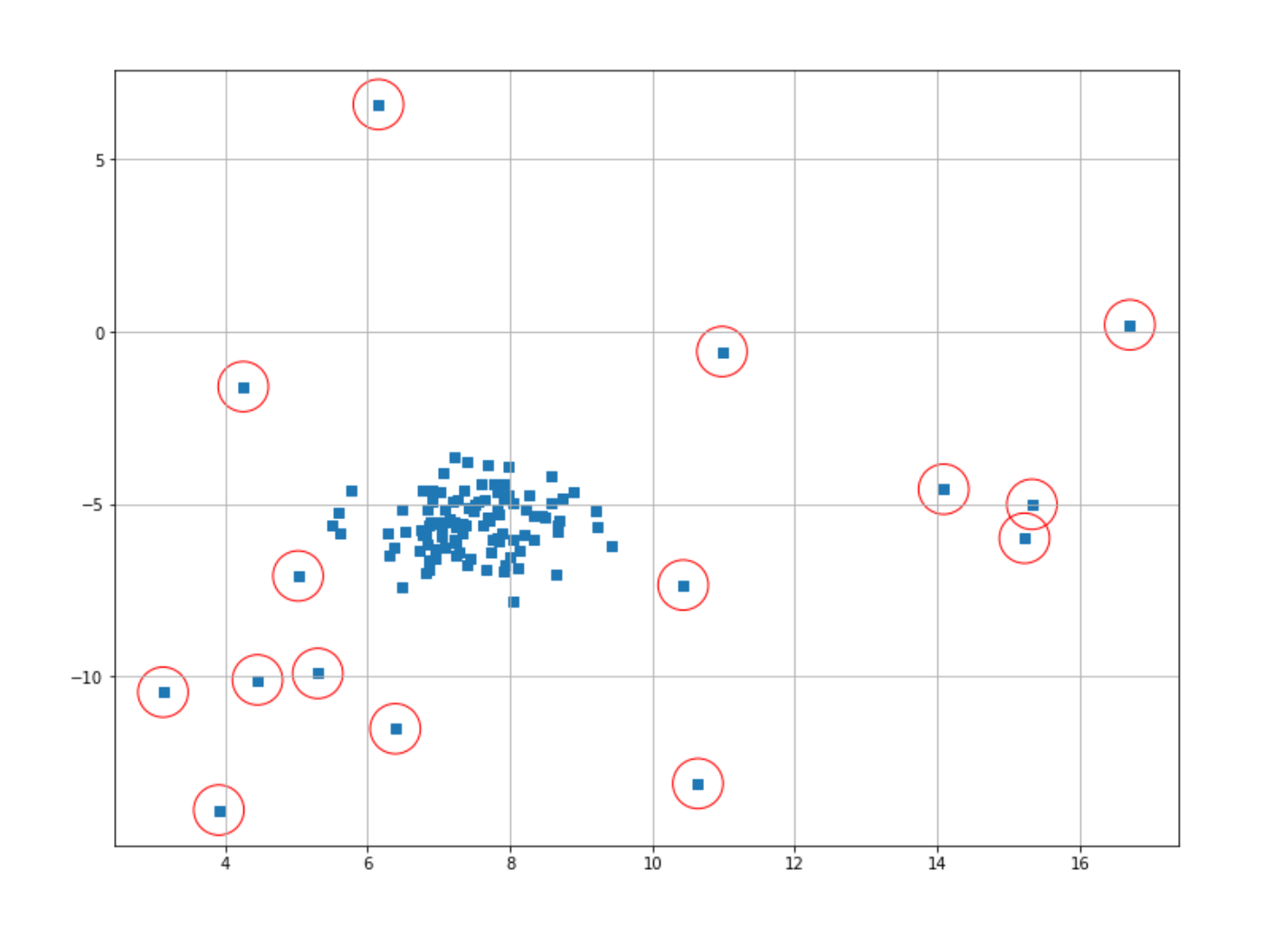
As you can see, now our One-Class SVM does a better job in determining the outliers compared to before, but not quite optimal yet. You can play around with the hyperparameter to find the best result. The main drawback of this algorithm is that this ⋎ value is difficult to optimize, and it generally doesn’t scale well when we have a lot more data points.
Conclusion
In this article, we have learned various machine learning algorithms commonly used for anomaly detection, such as Gaussian Mixture Model, Kernel Density Estimation, Isolation Forest, Local Outlier Factor, DBSCAN, and One-Class SVM. There is not one algorithm that is completely superior to the other, so in the end, you need to pick one algorithm that works the best for your use case.
As always, you can check out other articles on StrataScratch about an in-depth explanation of machine learning algorithms, for example:
- Machine Learning Algorithms that you should know → Machine Learning Algorithms
- If you want to learn more about Decision Tree and Random Forest, you can check out this article → Decision Tree and Random Forest Explained
- If you want to learn more about Clustering algorithm, you can check out this article → Machine Learning Clustering
- If you want to learn more about Classification algorithm, you can check out this article → Classification Machine Learning Algorithms
Share