Showing you what the cumulative sum is and how to calculate it in SQL. We’ll go through three distinct methods, so you can use whichever method you like best.

Cumulative sum is one of the common places in data analysis. SQL is also one of the common tools in extracting data from databases and analyzing it. From this, it follows that calculating cumulative sum is common in SQL. Yes, it is. We can confirm that!

Luckily, SQL allows you to calculate the cumulative sum relatively easily. Unfortunately for you, it’s not that easy if you don’t know how!

We’ll guide you through the logic of calculating the cumulative sum and how to apply this logic to SQL. Then we’ll go through several ways of computing the cumulative sum in SQL and show you how it’s done on one of our interview questions.

Let’s start with the foundations.

What is the Cumulative Sum in SQL?

A cumulative sum is calculated by adding all previous values in a sequence to the current value. The sequence is usually a date or time, so the cumulative sum gives you a sum at a certain time.

In SQL, this means accessing all the previous rows, summing them, and adding the sum to the current row’s value.

Imagine you’re working with the table showing the daily sales.

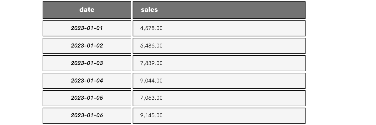
The cumulative sum for January 1 is 4,578.00, i.e., the same as the sales value for that date. The reason is there are no dates before that.

For January 2, the cumulative sum is the sum of January 1 and January 2 sales: 4,578.00 + 6,486.00 = 11,064.00.

You follow the same way until you reach the end of the table, as shown below.

Understanding the Importance of Cumulative Sums in Data Analysis

SQL cumulative sums play an essential role in data analysis. It allows you to track the accumulation of values over time.

This is helpful when wanting to identify trends and monitor growth or decline for various values important to businesses.

Based on that, you can also build different analytical views and data visualization. That way, you’re helping businesses make better decisions.

The cumulative sums also contribute to the creation of different analytical views of data and can provide insights for business decisions.

Step-by-Step Guide: Performing Cumulative Sum Calculations in SQL

There are several methods for calculating cumulative sums in SQL. We'll go through the three most common techniques.

Cumulative Sum Using Self Join

The self join method involves joining a table with itself. When doing that, you’re giving the table two different aliases. That way, you’re able to join the table with itself like it’s two different tables.

It’s also important to note that self join is not a special type of join – any type of join in SQL can be used for self joining the table.

We won’t go any further into explaining self joins, as you can learn more about it in our illustrated guide to self joins.

We’ll focus here on how to use self join to calculate the cumulative sum in SQL.

Example

We’ll use the question from Meta/Facebook to show you how this method works. However, we’ll change the question requirements.

Instead of calculating the cumulative sum over all three continents, we’ll do that only for Europe.

Dataset

The question gives you three tables to work with. Since we changed the question requirement, we’ll use only the table fb_eu_energy.

The table is simple – it shows the energy consumption for each date.

Code

Now, to calculate the cumulative energy consumption, let’s first join the table with itself.

SELECT
FROM fb_eu_energy eu1
JOIN fb_eu_energy eu2
ON eu1.date >= eu2.date;

We reference the table in FROM and give it an alias. Then we do the same in JOIN and give the table another alias. So, we’re pretending we have two different tables.

We’re joining the tables on the date column. However, not where the dates are the same. Remember, to calculate the cumulative sum for the current row, we need to access the values from all the previous rows. We achieve that by joining the table on the condition that the date from one table is equal to or greater than the date in another table.

Now we add the date and energy consumption in SELECT. Then we simply use the SUM() aggregate function – it allows us to find the sum, while the JOIN condition adds the cumulative aspect to it.

SELECT eu1.date,
       eu1.consumption,
       SUM(eu2.consumption) AS cumulative_consumption
FROM fb_eu_energy eu1
JOIN fb_eu_energy eu2
ON eu1.date >= eu2.date;

Finally, we group the output by the date and consumption. Adding ORDER BY and sorting the output ascendingly is also important – there’s no point in having a cumulative sum if the dates aren’t sorted, so the increase in the cumulative sum can be easily followed.

Our solution now looks like this.

SELECT eu1.date,
       eu1.consumption,
       SUM(eu2.consumption) AS cumulative_consumption
FROM fb_eu_energy eu1
JOIN fb_eu_energy eu2
ON eu1.date >= eu2.date
GROUP BY eu1.date, eu1.consumption
ORDER BY eu1.date;

Output

The output returns exactly what we wanted. You can check it manually, but it really shows the cumulative consumption.

Cumulative Sum Using Correlated Subquery

A subquery in SQL is a type of query that is written inside the other query. That’s why the subquery is also called an inner or nested query, and the query in which it is embedded is called an outer or main query.

A correlated subquery is a special type of subquery. Its specialness lies in the fact that it relies on the result returned by the main query. Also, it means that the subquery is evaluated repeatedly, once for each row returned by the main query.

The query from the previous example can be rewritten like this, so it uses the correlated subquery.

SELECT eu1.date,
       eu1.consumption,
  	 (SELECT SUM(eu2.consumption) 
  	  FROM fb_eu_energy eu2 WHERE eu1.date >= eu2.date) AS cumulative_consumption
FROM fb_eu_energy eu1
ORDER BY eu1.date;

The logic is similar as earlier, only this time we don’t use self join. However, we still use the same table twice.

The first time, it’s in the main query.

The second time, it’s in a subquery. This subquery uses SUM() to calculate the consumption sum. Then, WHERE uses the same condition we used in the ON clause in the previous example. Same as there, it looks for the dates in one table that are equal to or greater than the dates in the second table. This gives us cumulative, not the ‘regular’ sum.

Now that you know the logic of using a correlated subquery to get a cumulative sum, let’s try to solve the question without changing the requirements.

Example

It’s the same question from Meta/Facebook, only we’ll now do everything it asks.

We again have to calculate the cumulative sum. Now, it’s across the three continents. We have to output the dates and the cumulative sum rounded to the nearest whole number.

Dataset

The question’s full dataset consists of three tables. The first table is fb_eu_energy.

It shows energy consumption in Europe.

The next table is fb_na_energy, which shows energy consumption in North America.

The third table, fb_asia_energy, shows consumption in Asia.

Code

The code is much more complex than the previous one, so let’s break it down into parts.

To solve the question, we first need to consolidate all three tables into one. Since they all have the same columns, using UNION ALL within a CTE is the most efficient way.

WITH total_energy AS (
   SELECT *
   FROM fb_eu_energy eu

   UNION ALL 

   SELECT *
   FROM fb_na_energy

   UNION ALL 

   SELECT *
   FROM fb_asia_energy
)

Now we have all three tables shown as one. Let’s see the output using the following code.

SELECT *
FROM total_energy;

The output shows all dates and consumptions from all tables. Duplicates are not ignored because we used UNION ALL, not UNION.

Now we add the second CTE. We use it to reference the first CTE and calculate the energy consumption by date.

energy_by_date AS (
   SELECT date, 
   SUM(consumption) AS total_consumption
   FROM total_energy
   GROUP BY date
)

Let’s use the following code to see this CTE’s output.

SELECT *
FROM energy_by_date
ORDER BY date;

As you can see, it shows the dates and the energy consumption on each date. We used CTEs to prepare data. Now, we can go and calculate the cumulative energy consumption.

The final part of the code uses the correlated query to calculate the cumulative sum. The principle is the same as when we introduced you to this method.

Let’s explain this in several steps. First, select the date from the energy_by_date  CTE and give it an alias. Also, sort the output by dates ascendingly.

SELECT ebd1.date
FROM energy_by_date ebd1
ORDER BY ebd1.date;

Then, add the correlated query that calculates the cumulative sum. You should know how this works: use the SUM on the total_consumption column from the energy_by_date CTE. You’re using the same CTE in the main query, so give it another alias. Then filter data using WHERE, so the sum will be calculated for all the dates where the date from the main query is equal to or greater than the date from the subquery.

SELECT ebd1.date,
	 (SELECT SUM(ebd2.total_consumption)
   	  FROM energy_by_date ebd2
   	  WHERE ebd1.date >= ebd2.date) AS cumulative_consumption
FROM energy_by_date ebd1
ORDER BY ebd1.date;

Now, we also need to calculate the cumulative sum percentage and round it. It is calculated by dividing the cumulative sum by the total sum and multiplying by 100.

We simply copy the same correlated subquery we used above. Then we divide it by another subquery. This second subquery also references the energy_by_date CTE, and the product of division is multiplied by 100.

As we need to round the percentage to the nearest whole number, we use the ROUND() function with 0 as a decimals argument.

SELECT ebd1.date,
  	 (SELECT SUM(ebd2.total_consumption)
   	  FROM energy_by_date ebd2
   	  WHERE ebd1.date >= ebd2.date) AS cumulative_consumption,
       ROUND((SELECT SUM(ebd2.total_consumption)
              FROM energy_by_date ebd2
              WHERE ebd1.date >= ebd2.date) /
               (SELECT SUM(total_consumption)
                FROM energy_by_date)*100, 0) AS running_total_percentage
FROM energy_by_date ebd1
ORDER BY ebd1.date;

If we combine all these parts, we get this final code.

WITH total_energy AS (
  SELECT *
  FROM fb_eu_energy eu

  UNION ALL

  SELECT * 
  FROM fb_na_energy

  UNION ALL

  SELECT * 
  FROM fb_asia_energy
),

energy_by_date AS (
  SELECT date, 
         SUM(consumption) as total_consumption 
         FROM total_energy
         GROUP BY date
)

SELECT ebd1.date,
  	 (SELECT SUM(ebd2.total_consumption)
   	  FROM energy_by_date ebd2
   	  WHERE ebd1.date >= ebd2.date) AS cumulative_consumption,
       ROUND((SELECT SUM(ebd2.total_consumption)
              FROM energy_by_date ebd2
              WHERE ebd1.date >= ebd2.date) /
               (SELECT SUM(total_consumption)
                FROM energy_by_date)*100, 0) AS running_total_percentage
FROM energy_by_date ebd1
ORDER BY ebd1.date;

Output

Here’s what the code returns. As we intended, it shows the cumulative energy consumption and its percentage for each day.

Cumulative Sum Using OVER and ORDER BY CLAUSE

The easiest and, at the same time, the most complex way of calculating cumulative sum is by using the window function.

It’s the easiest because the code will have fewer lines. It’s the most complex because it requires, well, knowing window functions – they are hard before you learn them. Isn’t that the case with everything?

The window functions are functions that are applied to the rows that are somehow related to the current row. We call these rows a window, hence the window functions. If you feel your knowledge of the window functions is lacking, please read more in The Ultimate Guide to SQL Window Functions.

One of the important characteristics of the window functions is that they don’t collapse the individual rows when aggregating data. In other words, it allows us to show the individual and aggregated values at the same time. This important feature makes calculating cumulative sum much more efficient than in the previous examples.

We’ll use the SUM() aggregate window functions for our calculations. Yes, it sums values, just like a regular aggregate function. But with the window function features, it gets much more possibilities.

The two most important clauses for our calculation are OVER() and ORDER BY. The syntax of the window function we’ll use looks like this:

SELECT …, 
  	SUM(column_name) OVER (ORDER BY … ) AS cumulative_sum 
  FROM table;

Where:

• SUM(column_name) – Regular SUM() applied to a column.
• OVER – Mandatory clause that turns the function into a window function
• ORDER BY – Optional clause used for sorting the window frame, i.e., defining the calculation order. Note: Not the same as ORDER BY in SELECT, which is used for sorting the output.

Additional note: Depending on your task, you might also need to use PARTITION BY in OVER(). It is used for partitioning a window into smaller groups. For example, if you had a table showing consumption in Europe and several of its cities – PARTITION BY would allow you to calculate the cumulative sum for each city, not only for the whole continent. We have a nice explanation of PARTITION BY in our SQL cheat sheet.

Let’s use this syntax on a simplified version of our interview question. Again, we’ll calculate only the cumulative sum in Europe.

SELECT date, 
       consumption,
       SUM(consumption) OVER (ORDER BY date ASC) AS cumulative_consumption
FROM fb_eu_energy;

Instead of self joining or writing a subquery, we calculate the cumulative consumption much easier this way. So, we apply the SUM() function to the consumption column. Then we use the OVER() clause to turn it into a window function.

In OVER(), we use ORDER BY so that the cumulative sum is calculated from the oldest to the latest date. Which is exactly how it should be done.

Example

We’ll use the same Meta/Facebook interview question as earlier and solve it as it is.

Coding

In the previous example, we used the CTEs and a correlated subquery to solve the problem. This time, we’ll keep the CTEs. But instead of a subquery, we’ll use the window functions.

We can skip explaining the CTEs, as they are identical to the previous example.

WITH total_energy AS (
  SELECT *
  FROM fb_eu_energy eu
  UNION ALL
  SELECT * 
  FROM fb_na_energy
  UNION ALL
  SELECT * 
  FROM fb_asia_energy
),

energy_by_date AS (
  SELECT date, 
         SUM(consumption) as total_consumption 
         FROM total_energy
         GROUP BY date
)

SELECT date,
  	 SUM(total_consumption) OVER (ORDER BY date ASC) AS cumulative_consumption,
       ROUND(SUM(total_consumption) OVER (ORDER BY date ASC)/(SELECT SUM(total_consumption) FROM energy_by_date)*100, 0) AS running_total_percentage
FROM energy_by_date
ORDER BY date;

Now, the cumulative sum calculation is different – we use the power of the window functions. We apply the SUM() function to the total consumption from the energy_by_date CTE. Then, in the OVER() clause, we sort the window frame by date ascendingly, so the cumulative sum goes from the oldest to the latest date.

Now, we can calculate the percentage. The principle is the same as in the previous example when we solved the complete question: copy the cumulative calculation, divide it by the subquery that finds the total consumption (the same subquery as in the previous example), multiply by 100, and round to the nearest whole number.

Output

As you can see, the output is the same as in the previous example.

Optimizing Performance: Tips and Tricks for Efficient Cumulative Sum Computations in SQL

For large datasets, the performance of SQL cumulative sum calculations can become a concern. Here are some tips:

1. Use window functions: As shown above, window functions tend to be more efficient than self joins or subqueries.
2. Index your data: Properly indexing your data can speed up the computations.
3. Break down complex queries: If your cumulative sum involves complex conditions, breaking it down into smaller parts can help optimize the process.

Real-World Use Cases and Applications of Cumulative Sums in SQL

SQL cumulative sum is extensively used in various fields for different types of data analysis. Here are some real-world applications.

1. Finance and Accounting – cumulative sums of transactions, sales, costs, or other financial data over a certain period. They can help identify trends, such as sales growth or decline, over time. Depending on the decision, these trends can be monitored, for example, daily, monthly, or annually to check the performance and adjust strategies.

2. Inventory Management – tracking the quantity of inventory over time. By recording each addition or subtraction from inventory, a running total provides the current inventory level at any point in time.

3. Performance Monitoring – tracking the total number of errors logged in a system, the total downtime of a service over a period of time, or the number of hours worked. This can help in identifying patterns and making improvements.

4. Sports and Games – tracking the total points scored by a player or team over a season or career or ranking the players based on their cumulative scores.

5. Healthcare – the total number of cases of a disease over time in medical research or public health monitoring. It can be crucial in identifying and responding to outbreaks. Or counting the number of people infected by COVID-19; that was not that long ago.

6. Telecommunications – for calculating the total data used in a certain period, the total minutes a customer spent on calls, or the number of SMS they sent.

7. Website Analytics – for tracking the total number of page views, clicks, or other user interactions over a period.

8. Weather data analysis – used for calculating the cumulative rainfall in a particular region during a certain period, which can be useful in climate studies or planning agricultural activities.

Cumulative Sum Versus Running Total

While cumulative sum and running total might sound similar, they have slightly different applications.

Both calculations will return a cumulative result for a certain period. However, here’s the difference – defining the period.

The cumulative sum shows the cumulative result from the first date until today. As you go on, the time frame increases. For example, if you’re calculating daily cumulative revenue, with each day, your time frame increases by one day.

The running total, however, has a fixed size of a frame. However, the frame moves with each new period. Hence, ‘running’ in running total. In other words, running total looks at a certain time frame in history. For example, a 3-day running total revenue means that the running total will include the revenues of the last two days plus the current day. The next day, it will again include the same number of days. But they won’t be the same days as yesterday, as the time frame moves (not increases, moves!) along with the current date.

You can see how this works in the GIF below.

Yes, the first three running totals will be the same as the cumulative sum. But don’t be mistaken that this GIF is the same as the previous one!

After three days, the running total still keeps taking into account only the last three days, while the cumulative cum includes all the previous days.

Conclusion

The cumulative sum as a mathematical concept is rather simple. However, calculating it in SQL requires some advanced SQL techniques. It can seem complicated because of that. But, with a solid understanding of the language's concepts and the right techniques, you can easily translate the cumulative sum logic to SQL.

There are three distinct ways of calculating the cumulative sum in SQL, and they involve three important SQL topics: (self) joins, (correlated) subqueries, and window functions.

These concepts have a much broader application in SQL overall, so knowing them will help you in many more tasks other than the cumulative sum. Virtually no intermediate or advanced SQL queries can be written without these three concepts. Plenty of our interview questions require this knowledge, so we recommend using them for code practice.