Probability Cheat Sheet: Rules, Laws, Concepts, and Examples

What is Probability?

Let's begin our probability cheat sheet by exploring the concept of probability.

Definition: Probability is a mathematical concept for measuring the likelihood of an event occurring. In other words, probability quantifies how likely an event is to occur on a scale from 0 to 1. Zero means impossibility, and 1 indicates certainty. Probability is expressed as a fraction, decimal number, or percentage.

Formula: The probability of an event occurring is calculated like this.

P = \frac{Number\ of\ Favorable\ Outcomes}{Total\ Number\ of\ Outcomes}

Example: In flipping a coin, these are the values for calculating the probability of getting a head.

Number of Favorable Outcomes = 1 (there’s one head)
Total Number of Outcomes = 2 (there’s one head and one tail)

The probability is:

P = \frac{Number\ of\ Favorable\ Outcomes}{Total\ Number\ of\ Outcomes} = \frac{1}{2} = 0.5 = 50\%

What Are the Rules of Probability?

Next, we will explore the rules in our probability cheat sheet.

Definition: The probability rules are the basic principles defining the foundation of probability.

1. Addition Rule

Definition (mutually exclusive events): The exclusive events are those that can’t occur at the same time. The probability of the occurrence of one event or another event, in that case, is the sum of their individual probabilities.

Formula (mutually exclusive events):

P(A\cup B) = P(A) + P(B)

Note:

P(A\cup B)\ = P(A\ or\ B)

Example (mutually exclusive events): Consider a single tossing of a coin. When you’re tossing it, two events can occur:

A = getting head
B = getting tails

We can calculate the probability of getting head or tails in one coin toss. Let’s first calculate the probability for each event.

P(head) = P(A) = \frac{Number\ of\ Favorable\ Outcomes}{Total\ Number\ of\ Outcomes} = \frac{1}{2} = 0.5 = 50\%

P(tails) = P(B) = \frac{Number\ of\ Favorable\ Outcomes}{Total\ Number\ of\ Outcomes} = \frac{1}{2} = 0.5 = 50\%

Use these values in the probability formula. The probability of getting head or tails in one coin toss is 100%.

P(head\cup tails) = P(A\cup B) = P(A) + P(B) = \frac{1}{2} + \frac{1}{2} = 1 = 100\%

Definition (mutually non-exclusive events): The two events are mutually exclusive if they can occur simultaneously. In that case, the probability of either event occurring is the sum of their individual probabilities minus the probability of both events occurring together.

Formula (mutually non-exclusive events):

P(A\cup B) = P(A) + P(B) - P(A\cap B)

Note:

P(A\cap B) = P(A\ and\ B)

Example (mutually non-exclusive events): In this question by Meta, you need to calculate the probability of pulling a different color or shape card from a shuffled deck of 52 cards.

Probability Cheat Sheet Interview Question

Pulling a card of a different color or shape are mutually non-exclusive events. We’ll call them events A and B:

A = probability of selecting a card with a different color
B = probability of selecting a card with a different shape

Let’s calculate the probability of event A. A deck of cards has 52 cards; 26 are black, 26 are red. If we pull one card out randomly, 26 cards of the other color will still be left, i.e., the number of favorable events. In total, there are 51 cards left, i.e., the total number of outcomes.

P(A) = \frac{Number\ of\ Favorable\ Outcomes}{Total\ Number\ of\ Outcomes} = \frac{26}{51} = 0.5098 = 50.98\%

Now, the probability of event B. Before drawing a card, there are 13 cards of each of the four shapes: clubs, diamonds, hearts, and spades. After we draw one card, there are 3 remaining different shapes, each with 13 cards. Again, 51 cards left is after one drawing.

P(B) = \frac{Number\ of\ Favorable\ Outcomes}{Total\ Number\ of\ Outcomes} = \frac{3*13}{51} = \frac{39}{51} =\frac{13}{17} = 0.7647 = 76.47\%

Now, we need the probability of pulling a second card of different colors and shapes. In other words, the probability of events A and B occurring at the same time. Two shapes (spades and clubs) are black, and two (hearts and diamonds) are red. With drawing, there remain only two other shapes with 13 cards each that are of different colors. The total number of outcomes is 51.

P(A\cap B) = \frac{Number\ of\ Favorable\ Outcomes}{Total\ Number\ of\ Outcomes} = \frac{2*13}{51} = \frac{26}{51} = 0.5098 = 50.98\%

So, to answer the question, we need to plug these values into the mutually non-exclusive events probability formula. The probability of pulling a different color or shape card from a shuffled deck of 52 cards is 76.47%.

P(A\cup B) = P(A) + P(B) - P(A\cap B) = \frac{26}{51} + \frac{39}{51} - \frac{26}{51} = \frac{39}{51} = \frac{13}{17} = 0.7647 = 76.47\%

2. Rule of Complementary Events

Definition: The probability of an event not occurring is equal to one minus the probability of that event occurring. In other words, the sum of the probabilities of an event and its complement (the event not happening) is always one.

Formula:

P(A') = 1 - P(A)

A’ = The complement of the event A, i.e., the event A not occurring

Example: Let’s modify this question by Belvedere Trading a little. Sure, we’ll calculate the probability of getting a 6 when rolling a die. But we’ll also use the rule of complementary events to calculate the probability of not getting a 6.

Probability Cheat Sheet Interview Question 2

A dice has six sides, so the total number of outcomes is 6. We want to get the number 6 when rolling a die, so the number of positive outcomes is 1.

P(A) = \frac{Number\ of\ Favorable\ Outcomes}{Total\ Number\ of\ Outcomes} = \frac{1}{6} = 0.1667 = 16.67\%

So, 16.67% is the probability of getting the number 6. This answers the interview question.

Let’s now use the complementary rule to answer our additional question.

P(A') = 1 - P(A) = 1 - \frac{1}{6} = \frac{5}{6} = 0.8333 = 83.33\%

This result means that the probability of not getting a 6 when rolling a die is 83.33%.

3. Rule of Conditional Probability

Definition: The rule of conditional probability explains the probability of an event occurring, given that another event has already occurred.

In other words, it describes how the likelihood of an event might change based on the occurrence of a related event. Under conditional probability, we're interested in the probability of one event (Event A) happening if a related event (Event B) has already taken place.

With this rule, we can adjust our calculations based on the new information provided by the occurrence of Event B.

Formula:

P(A\ |\ B) = \frac{P(A\ \cap\ B)}{P(B)}

Note:

P(A\ |\ B) = P(A\ given\ B)

Example: This is a question from the Goldman Sachs interview. It gives you its own definitions of certain values that we can use to calculate the probability that Company X goes bankrupt before T.

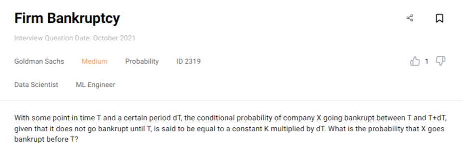
Probability Cheat Sheet Interview Question 3

It’s a conditional probability. We can use the above formula to plug in all the values given to us by the question.

Let’s first define the events.

A = company X goes bankrupt between T and T+dT
B = company X doesn’t go bankrupt until T

The question asks to find the probability that the company does go bankrupt. It’s a complementary event to the event B. So, we want to find P(B’).

The question defines the conditional probability as K*dT. Therefore:

P(A\ |\ B) = K*dT

So, the probability of the complementary event is this.

P(B') = 1-P(B)

From that, we know this is also true.

P(B) = 1-P(B')

Again, this is the conditional probability formula.

P(A\ |\ B) = \frac{P(A\ \cap\ B)}{P(B)}

Let’s plug the above values into it.

K*dT = \frac{P(A\ \cap\ B)}{1-P(B')}

From there, we can get P(B’). It’s the probability that Company X will go bankrupt before T.

P(B') = \frac{K*dT - P(A\ \cap\ B)}{K*dT}

4. Multiplication Rule

Definition (independent events): The multiplication rule determines the probability of two events happening together. If the two events are independent, then the occurrence of one doesn’t influence the occurrence of the other. In that case, the probability of both events happening together is the product of their individual probabilities.

Formula (independent events):

P(A\cap\ B) = P(A)\cdot P(B)

Example: Let’s assume that you’re tossing a coin. You want to calculate the probability of getting tails in two consecutive tosses. These events are independent, as getting tails the first time doesn’t change the probability of getting tails the second time.

So the probability is 25%.

P(A\cap\ B) = P(A)\cdot P(B) = \frac{1}{2}\cdot\frac{1}{2} = \frac{1}{4} = 0.25 = 25\%

Definition (dependent events): Two events are dependent when the occurrence of one does influence the occurrence of the other event. In that case, the probability of both events happening together is the product of the probability of the first event and the conditional probability of the second event, given that the first event has occurred.

Formula (dependent events):

P(A\ \cap\ B) = P(A)\cdot P(B\ |\ A)

Example: Here’s a question that appeared in the Zenefits, Pinterest, and Quora interviews.

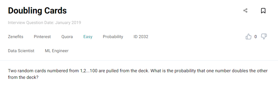
Probability Cheat Sheet Interview Question 4

We need to calculate the probability that one number will double the other if we pull two random cards numbered from 1 to 100.

First, let’s define the events.

X1 = the number of the first card pulled from the deck
X2 = the number of the second card pulled from the deck

There are two scenarios when one number will double the other.

Scenario 1: The second card is double the value of the first card. For that to happen, X1 has to belong to the set {1, 2, …, 50}, so:

X_2 = 2*X_1

Otherwise, X2 can’t be a double of X1.

Scenario 2: The second card is half the value of the first card. This means that X1 had to be an even number, i.e., divisible by 2. In that case,

X_1 = 2*X_2

From the two scenarios come the following events.

A = X1 belongs to the set {1, 2, …, 50}
B = X1 is an even number
C = X2 is double the value of X1
D = X2 is half the value of X1

We’ll now calculate the probability for each of the two scenarios separately.

Scenario 1: This scenario involves dependent events A and C. We’ll use the multiplication rule to get the probability the following way. There are 50 positive outcomes for the A event. Given A, there’s only one positive outcome for event C, i.e., only one card (of the remaining 100) can be double the value of the first card.

P(second\ card\ doubles\ the\ first\ card) = P(2*X_1 = X_2) = P(A)\cdot P(C\ |\ A) = \frac{50}{100}\cdot \frac{1}{99} = \frac{50}{9900} = \frac{1}{198}

Scenario 2: In this scenario, we have events B and D. We’ll apply the same formula as in the previous scenario. Again, there will be 50 positive outcomes for the event B. Given B, there’s only one card that can be half the value of the first card, i.e., one positive outcome for event D.

P(second\ card\ is\ half\ the\ first\ card) = P(X_1 = 2*X_2) = P(B)\cdot P(D\ |\ B) = \frac{50}{100}\cdot \frac{1}{99} = \frac{50}{9900} = \frac{1}{198}

To answer the question, we need to sum the probabilities of Scenario 1 and Scenario 2 using the addition rule.

P(one\ card\ doubles\ the\ other\ from\ the\ deck) = P(Scenario\ 1) + P(Scenario\ 2) = \frac{1}{198} + \frac{1}{198} = \frac{2}{198} = \frac{1}{99} = 0.0101 = 1.01\%

If we pull two random cards numbered from 1 to 100, there’s a 1.01% probability that one card will be double the other.

What Are the Laws of Probability?

Next on our Probability cheat sheet, here are the laws of Probability you should be familiar with.

Definition: The laws of probability are the more advanced principles derived from the basic rules of probability.

Bayes’ Theorem

Definition: Bases’ theorem is a conditional probability statement that defines the probability of an event happening, given that another event related to the first one has already happened.

Formula: The Bayes’ theorem formula is given below.

P(A\ |\ B) = \frac{P(B\ |\ A)*P(A)}{P(B)}

P(A | B) = the posterior probability or the probability of the event A occurring given that the event B has happened
P(B | A) = the likelihood or the probability of the event B occurring given that the event A has happened
P(A) = the prior probability or the initial probability of the event A
P(B) = the marginal likelihood or the total probability of the event B occurring

If the normalizing constant P(B) is not given, you can use this Bayes theorem version.

P(A\ |\ B) = \frac{P(B\ |\ A)*P(A)}{P(B\ |\ A)*P(A) + P(B\ |\ \neg A)*P(\neg A)}

Example: Here’s an interview question from Zenefits, AXA, and MetLife that requires you to know Bayes’ theorem.

Probability Cheat Sheet Interview Question 5

We need to calculate the probability of a stock actually going up when the program predicts it will go up.

Here, P(A) is the prior probability that the stock is going up. It will go up, or it won’t, so the probability is 0.5.

P(B | A) is the likelihood that the stock will go up when the program says so. The program’s accuracy rate is 60% or 0.6; this is our probability in this case.

P(B) is the probability that the program will say the stock will go up. We don’t have this value, so we have to use the modified version of Bayes’ theorem.

P(A\ |\ B) = \frac{P(B\ |\ A)*P(A)}{P(B\ |\ A)*P(A) + P(B\ |\ \neg A)*P(\neg A)}

We know that the probability of the program predicting the increase in value when the stock actually goes down is calculated like this. Remember the rule of complementary events?

P(B\ |\ \neg A) = 1 - P(B\ |\ A) = 1 - 0.6 = 0.4

We apply the same rule to get the probability of event A not happening, i.e., the stock goes down.

P(\neg A) = 1 - P(A) = 1 - 0.5 =0.5

Now, we can plug all this into the Bayes’ theorem formula.

P(A\ |\ B) = \frac{0.6*0.5}{0.6*0.5 + 0.4*0.5} = \frac{0.3}{0.3 + 0.2} = \frac{0.3}{0.5} = 0.6 = 60\%

In plain English, the probability for the stock to go up when the program says it will go up is 60%.

Law of Total Probability

Definition: It’s a law that calculates the probability of an event by considering all the ways it can happen based on a partition given by another event. In other words, you sum up the probabilities of B occurring given each event Ai, weighted by the probability of each Ai.

Formula: Translated into a formula, the law of total probability is expressed like this.

P(B) = \sum_{i=1}^{n}P(B\ |\ A_i) * P(A_i)

Example: The classic example of total probability is a disease that affects 2% of the population. The test for having a disease has the following characteristics:

If a person has a disease, the test will correctly identify them as positive 90% of the time.
If a person doesn’t have a disease, the test will falsely identify them as positive 3% of the time.

What is the probability that the random person tested positive?

For this, we need to use the law of total probability. There is one event B, and two events A:

B = the person tested positive
A1 = the person has the disease
A2 = the person doesn’t have a disease

The two possible outcomes in case of a positive test are:

The person has the disease and tests positive.
The person doesn’t have the disease but tests positive.

The values we need for the calculation are:

P(A1) = the probability of having the disease
P(A2) = the probability of not having the disease
P(B|A1) = the probability of testing positive and having the disease
P(B|A2) = the probability of testing positive and having the disease

The calculation will look like this.

P(B) = \sum_{i=1}^{n}P(B\ |\ A_i) * P(A_i) \\ \ \\ = P(B\ |\ A_1) * P(A_1) + P(B\ |\ A_2) * P(A_2) \\ \ \\ = 0.9 * 0.02 + 0.03 * (1 - P(A_1)) \\ \ \\ = 0.9 * 0.02 + 0.03 * 0.98 \\ \ \\ = 0.0180 + 0.0294 \\ \ \\ = 0.0474 \\ \ \\ = 4.74\%

So, the probability that the random person tests positive is 4.74%.

Probability Distributions

Definition: A probability distribution is a mathematical representation of the probabilities of all possible outcomes for a random variable in a given scenario. In other words, it defines how the likelihood of each possible outcome is distributed across the range of values that the random variable can take.

Discrete Probability Distributions

Definition: Discrete probability distributions describe the probabilities that the event outcome will take one of the values in a discrete set. Discrete value is the one that takes a certain countable and finite or countably infinite value, commonly expressed as a whole number or integer.

Important probability concepts:

PMF: Discrete probability distributions are defined by the Probability Mass Function (PMF). It assigns a probability to each possible outcome.

CDF: If calculating the probability that the variable will take on a value less than or equal to a given value, you should use the Cumulative Distribution Function (CDF). This is useful also when you want to find the probability of a variable taking on a value from the defined range.

It is given by this formula:

F_X(x) = P(X \leq x)

To find the probability that the random variable takes value from the interval, use this formula.

P(a<X\leq b) = F_X(b) - F_X(a)

Mean or Expected Value: The mean is the average value of a random variable. If taking many measurements from the probability distribution, the mean would represent a long-term average or expected value.

Median: The median is the middle value of the dataset arranged in ascending order. In the probability distribution, this means that half of the probability mass lies to the left of the median and half to the right of it.

Discrete Uniform Distribution

Definition: The discrete uniform distribution means that every outcome within a sample is equally likely to occur.

Formulas: The PMF of the uniform distribution is calculated in the following way.

f(x) = P(X = x) = \frac{1}{n}

X = the random variable
x = a particular outcome
n = the total number of equally likely outcomes

The CDF formula looks like this.

F(x) = \begin{cases} 0, &\quad \text{if}\ x < a \\ \frac{x-a+1}{n}, &\quad \text{if}\ a\leq x \leq b \\ 1, &\quad \text{if}\ x > b \end{cases}

a = the minimum value of the random variable
b = the maximum value of the random variable

The mean or expected value is given by this formula.

E(X) = \mu =\frac{a+b}{2}

The median is the same as mean.

\tilde{x} =\frac{a+b}{2}

Curve: The curve of the uniform distribution looks like this.

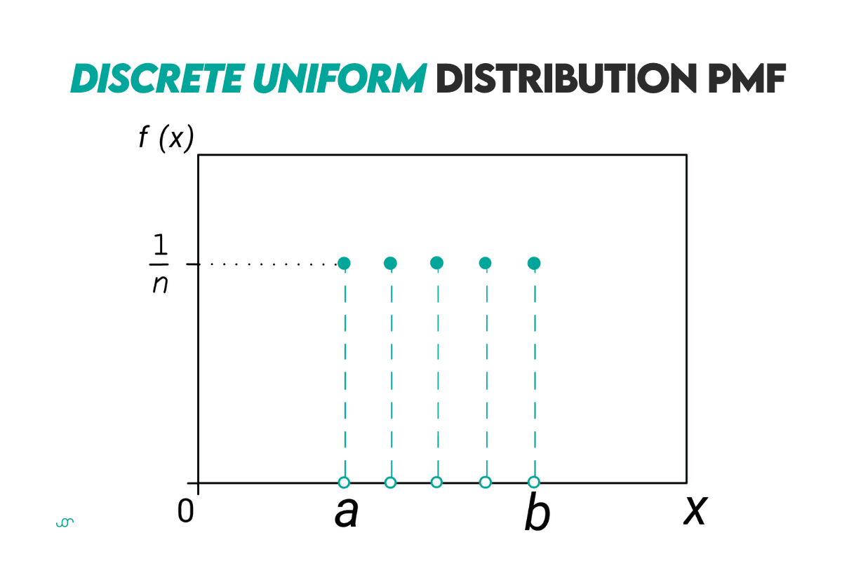
Discrete Uniform Distribution in Probability Cheat Sheet

Example: If you have a six-sided die, then n = 6. So the probability of getting any of six sides, e.g., 3, is 16.67%

P(X = 3) = \frac{1}{n} = \frac{1}{6} = 0.1667 = 16.67\%

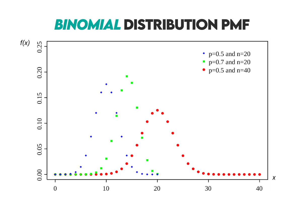
Binomial Distribution

Definition: It describes the number of successes in a fixed number of independent trials, i.e., Bernoulli trials. There are only two possible outcomes of each trial: success or failure.

Formulas: The binomial distribution has two parameters. The first one is the number of trials, n. The second one is the probability of success in a single trial, p. Here, the p is constant.

Here’s the PMF formula.

P(X = k) = \binom{n}{k}p^k(1-p)^{n-k}

P(X = k) = the probability of observing k successes in n trials
nk = the binomial coefficient; the number of ways to choose k successes from n trials
p = the probability of success on a single trial
(1-p) = the probability of failure on a single trial
n = the total number of trials
k = the number of successes; can take values from to 0 to n

Note: The binomial coefficient is calculated the following way.

\binom{n}{k} = \frac{n!}{k!(n-k)!}

The CDF is calculated this way.

F(x) = P(X\leq x) = \Sigma_{k=0}^{x}\binom{n}{k}p^k(1-p)^{n-k}

If you’re doing the same for the interval, just sum the CDFs for each value in the interval.

The expected value formula is given below.

E(X) = \mu = n*p

Regarding the median, there’s no unique formula. If n*p is an integer, then the median is the same as the mean.

\tilde{x} = n*p

If it’s not an integer, then you need to find the CDF for each k number of successes. The one that gets the closest to 0.5 is your median.

Curve: Here’s the binomial distribution curve shown with the normal distribution.

Binomial Distribution in Probability Cheat Sheet

Example: We can use the binomial distribution formula to solve this question asked by Microsoft, Apple, and IBM.

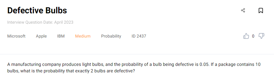
Probability Cheat Sheet Interview Question 6

Given the probability of a bulb being defective, we need to calculate the probability of 2 out of 10 bulbs being defective. Again, this is the formula we’ll use.

P(X = k) = \binom{n}{k}p^k(1-p)^{n-k}

Let’s define the values so we can plug them into the formula.

n = the total number of bulbs is 10
k = the number of defective bulbs is 2
p = the probability of a bulb being defective is 0.05
nk = the binomial coefficient showing the number of ways to choose two defective bulbs from the package of ten

With these values, the probability formula looks like this.

P(X = 2) = \binom{10}{2}0.05^2(1-0.05)^{10-2}

Let’s first calculate the binomial coefficient.

\binom{10}{2} = \frac{10!}{2!(10-2)!} = \frac{10!}{2!*8!} = 45

We’ll now use this value to get the answer to the question.

P(X = 2) = 45*0.05^2*0.95^8 = 0.0746 = 7.46\%

So the probability that two out of ten bulbs are defective is 7.46%.

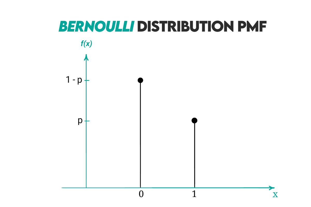
Bernoulli Distribution

Definition: The Bernoulli distribution is a special case of the binomial distribution where the number of trials is 1.

Formulas:

P(X = x) = p^x(1-p)^{1-x}

P(X = x) = the probability that the random variable X takes on the value x
p = the probability of success, i.e., X = 1
x = it can be either 0 (failure) or 1 (success)

Since x can have only two values, from this follows that there are two (shorter) formulas for Bernoulli distribution:

1. When x = 1 (success):

P(X = 1) = p

2. When x = 0 (failure):

P(X = 0) = 1 - p

Now, here’s the CDF that gets these values in three scenarios.

F(x) = \begin{cases} 0 & \text{if } x < 0 \\ 1-p & \text{if } 0 \leq x < 1 \\ 1 & \text{if } x \geq 1 \end{cases}

The expected value for Bernoulli distribution is:

E(X) =\mu = p

Regarding the median, it’s the same as the value x. There are two cases:

If p ≥ 0.5, the median is 1.
If p < 0.5, the median is 0.

Curve: Here’s the distribution curve.

Bernoulli Distribution in Probability cheat sheet

Example: Here’s a simple example from Belvedere Trading. We’ll solve it using the Bernoulli distribution.

Probability Cheat Sheet Interview Question 7

We need to calculate the probability of getting 6 from one roll of a dice. For the Bernoulli distribution, this means:

P(X = 1) = the probability of success, i.e., getting 6
P(X = 0) = the probability of all other outcomes

We know what the formula is in the case of success. The probability of getting a 6 is 1/6 since there is one favorable outcome out of six.

P(X = 1) = p =\frac{1}{6} = 0.1667 = 16.67\%

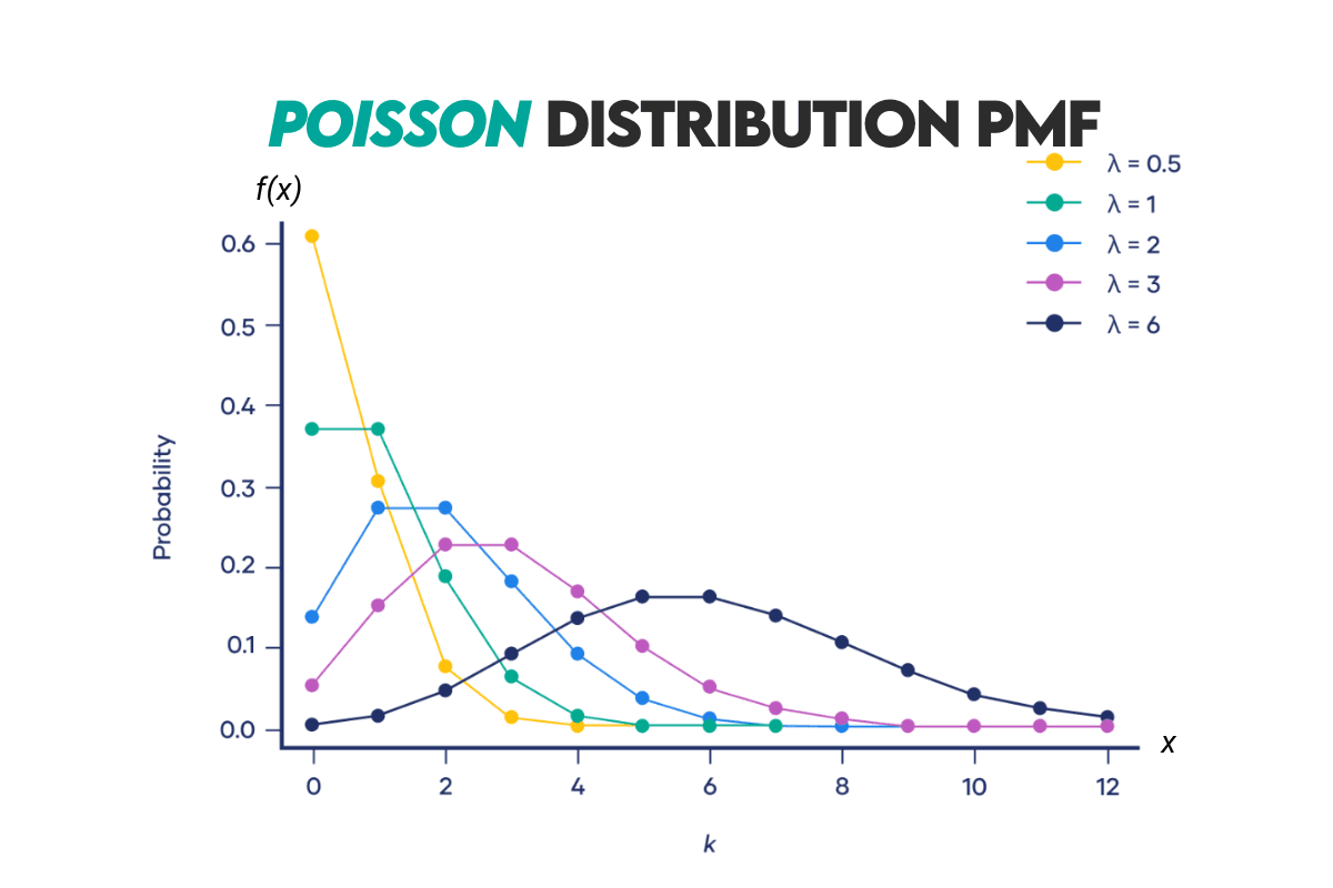
Poisson Distribution

Definition: It’s a distribution that describes the number of events in a fixed interval of time or space if these events occur with a known average rate and independently of the time since the last event.

Formula: Here’s the formula for calculating Poisson’s PMF.

f(x) = P(X = x) = \frac{\lambda^x e^{-\lambda}}{x!}

P(X = x) = the probability of observing x events
λ = the average rate (or mean) of occurrences in the given interval
e = the base of the natural logarithm ≈ 2.71828
x = non-negative integer (0, 1, 2, …)

The CDF of this distribution is given here.

F(x) = \sum_{i=0}^{\lfloor x \rfloor} \frac{\lambda^i e^{-\lambda}}{i!}

i = non-negative integer values

The ‘incomplete square brackets’ around x are called the floor function. You can read more about it here.

The expected value for this distribution is calculated like this.

E(X) = \mu = \lambda

The median is approximated using the following formula.

\tilde x \approx \lfloor \lambda + \frac{1}{3} - \frac{1}{50\lambda}\rfloor

Curve: Here’s the Poisson distribution curve.

Poisson Distribution in Probability Cheat Sheet

Example: We’ll use the example that appears in the official solution of this problem from Google and Amazon interviews.

Probability Cheat Sheet Interview Question 8

We want to calculate the probability of a football team scoring a specific number of goals in a match, given the average number of goals they score per match. If a team has an average of 1.5 goals per match, we want to calculate the probability of them scoring 3 goals in a match.

From this, we know that:

λ = 1.5
x = 3

Plug these values into the Poisson formula, and you get that the probability of the team scoring 3 goals in a match is 12.55%.

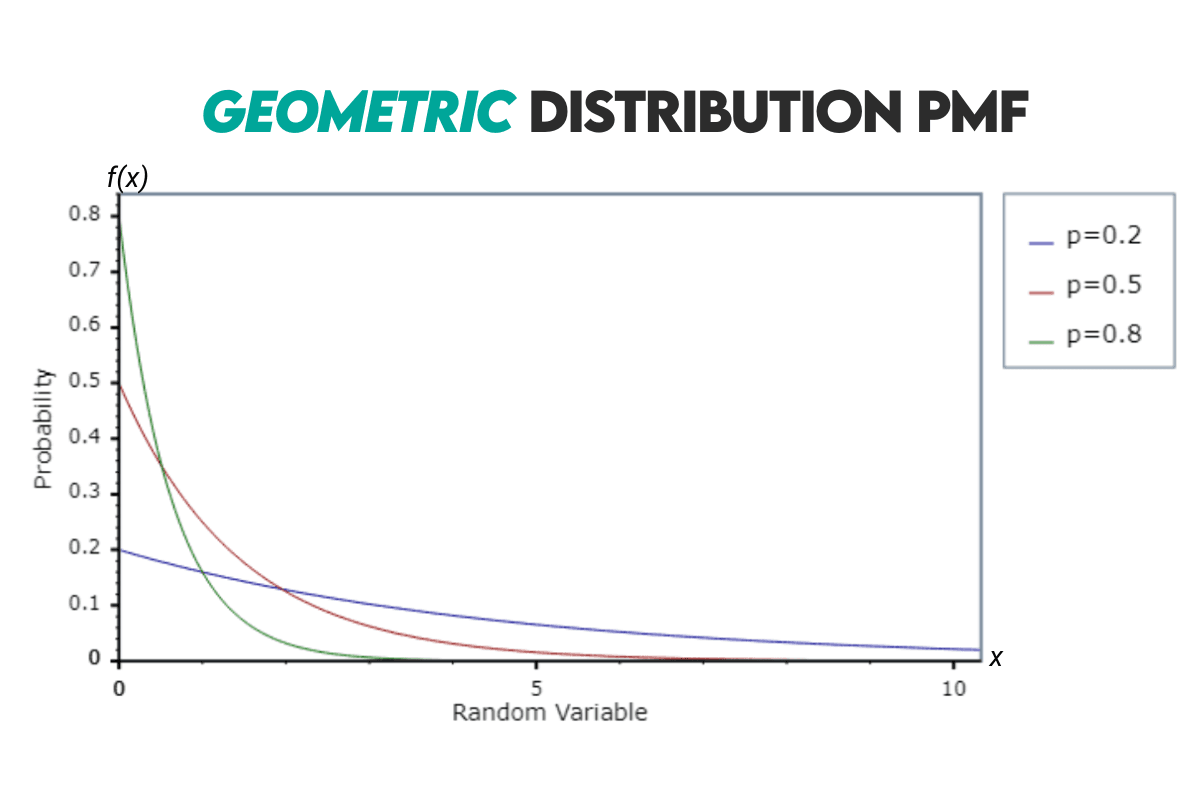
P(X = 3) = \frac{1.5^3 e^{-1.5}}{3!} =\frac{3.375 * 0.22313}{6} = 0.1255 = 12.55\%

Geometric Distribution

Definition: It represents the number of Bernoulli trials required for success to occur. Theoretically, the trials can go on indefinitely.

Formulas: The PMF formula is given below.

f(x) = P(X = x) = p(1-p)^{x-1}

p = the probability of success on any given trial

The CDF formula for the geometric distribution looks like this.

F(x) = 1 - (1-p)^x

When calculating the expected value, use the following formula.

E(X) = \mu = \frac{1}{p}

You’ll get the median of a geometric distribution with this formula.

\tilde x = \lceil \frac{-1}{log_2(1-p)}\rceil

Curve: The geometric distribution curve looks like this.

Geometric Distribution in Probability Cheat Sheet

Example: Let’s solve this interview question by Meta.

Probability Cheat Sheet Interview Question 9

We basically need to find the number of rolling two dice and getting 5. We’ll also calculate the expected earnings.

The number of possible outcomes with two dices on a single roll is:

Possible\ outcomes = 6*6 = 36

There are four ways in which you can get a sum of 5, i.e., win the game:

Getting 1 on the first die and 4 on the second die = {1, 4}
Getting 2 on the first die and 3 on the second die = {2, 3}
Getting 3 on the first die and 2 on the second die = {3, 2}
Getting 4 on the first die and 1 on the second die = {4, 1}

From there, the probability of winning in a single roll is:

p = \frac{Number\ of\ Positive\ Outcomes}{Total\ Number\ of\ Outcomes} = \frac{4}{36} = \frac{1}{9} = 0.1111 = 11.11\%

The expected number of rolls is:

E(X) = \frac{1}{p} = \frac{1}{\frac{1}{9}} = 9

This means that, on average, you can expect to roll the dice 9 times for you to win.

The question doesn’t require this, but let’s calculate the probability of winning in 9 rolls.

P(X = 9) = p(1-p)^{x-1} = \frac{1}{9}*(1-\frac{1}{9})^{9-1}= \frac{1}{9}*\left(\frac{8}{9}\right)^8 = 0.0433 = 4.33\%

Now we can go back to the expected number of rolls and calculate the expected earning. The income is defined as earnings minus expenses. We will calculate our income after 9 rolls. Each roll costs $5, and we win, we win $10.

Income = Earnings - Expenses = 10 * (number\ of\ wins) - 5*(number\ of\ rolls) = 10*1 - 5*9 = 10 - 45 = -35

This game doesn’t pay off for you, and your loss will be $35.

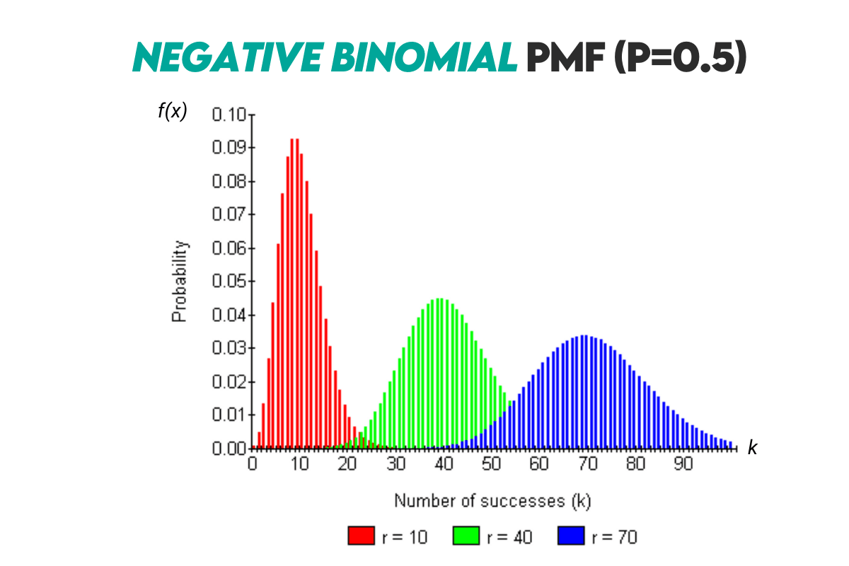
Negative Binomial Distribution

Definition: The negative binomial distribution is similar to the geometric distribution, but it counts the number of Bernoulli trials needed for a specified number of successes to occur.

Formula:

f(k) = P(X = k) = \binom {k-1}{r-1}p^r(1-p)^{k-r}

P(X = k) = the probability of observing r successes on the kth trial
p = the probability of success on any given trial
k = the total number of trials, where k is a positive integer and k ⩾ r
r = the specified number of successes, it has to be a positive integer
k-1r-1 = a binomial coefficient

The binomial coefficient is calculated the following way.

\binom {k-1}{r-1} = \frac{(k-1)!}{(r-1)!(k-r)!}

To calculate CDF, you will need this formula.

F(x) = I_p(r, k+1)

Ip(r, k+1) = the regularized incomplete beta function

The regularized incomplete beta function is calculated like this.

I_p(r, k+1) = \frac{\Beta (p;\ r,\ k + 1)}{\Beta(r,\ k + 1)}

B(p; r, k+1) = the incomplete beta function
B(r, k+1) = the beta function

You can read more about beta and incomplete beta functions and how to calculate them here.

The expected value of the negative binomial distribution is:

E(X) =\mu = \frac{r}{p}

Here’s also a formula for the median.

\tilde{x} = \begin{cases} \frac{k-1}{p} & \text{if } k \text{ is even} \\ \frac{k}{p} & \text{if } k \text{ is odd} \end{cases}

Curve: Here’s the curve for this distribution.

Negative Binomial Distribution in Probability Cheat Sheet

Example: Let’s solve the interview question by Chicago Trading Company.

Probability Cheat Sheet Interview Question 10

The probability of getting a head in a single toss is:

p = \frac{Number\ of\ Positive\ Outcomes}{Total\ Number\ of\ Outcomes} = \frac{1}{2} = 0.5 = 50\%

The number of successes (r) is 2. We can now use these values to calculate the expected number of tosses.

E(X) = \frac{r}{p} = \frac{2}{\frac{1}{2}} = 4

The answer to the question is that we can expect to toss the coin four times to get two heads.

Now, let’s find the probability of getting two heads after four tosses. The question does not require this, but let’s do it anyway.

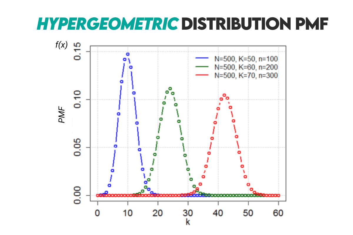
P(X = k) = \binom {k-1}{r-1}p^r(1-p)^{k-r} \\ \ \\ P(X = k) = \frac{(k-1)!}{(r-1)!(k-r)!}p^r(1-p)^{k-r} \\ \ \\ P(X = k) = \frac{(4-1)!}{(2-1)!(4-2)!}*\left(\frac{1}{2} \right)^2*(1-\frac{1}{2})^{4-2} \\ \ \\ P(X = k) = 3*\frac{1}{4}*\frac{1}{4} \\ \ \\ P(X = k) = \frac{12}{64} \\ \ \\ P(X = k)= \frac{3}{16} \\ \ \\ P(X = k) = 0.1875 \\ \ \\ P(X = k) = 18.75\%

Hypergeometric Distribution

Definition: It describes the probability of k number of successes in n number of draws without replacement from a finite population containing a specific number of successes.

Formulas: Here’s the PMF formula for the hypergeometric distribution.

f(x) = P(X = k) = \frac{\binom{K}{k}\binom{N-K}{n-k}}{\binom{N}{n}}

N = the total number of items in the population
K = the total number of successes in the population
n = the number of items drawn from the population
k = the number of successes among the drawn items

The CDF formula is this.

F(x) = \sum_{i=0}^x= \frac{\binom {K}{i}\cdot \binom {N-K}{n-i}}{\binom {N}{n}}

x = a non-negative integer representing the number of items with the desired characteristic in the sample

The expected value is calculated in the following way.

E(X) = \mu = \frac{nK}{N}

And finally, the median for the hypergeometric distribution.

\tilde x = \begin{cases} \frac{nK}{N}\quad &\text {if}\ n\leq K\\ n\quad &\text {if}\ n > K \end{cases}

Curve: Here’s the probability distribution curve.

Hypergeometric Distribution in Probability Cheat Sheet

Example: This question by Goldman Sachs can be solved using the hypergeometrical distribution.

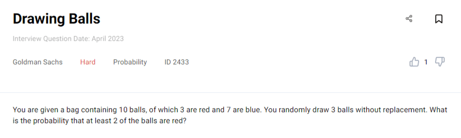
Probability Cheat Sheet Interview Question 11

You need to find the probability of getting at least two balls when drawing three balls from the bag of ten balls.

The values we get from the question that we’ll use in the hypergeometrical distribution formula are:

N = the total number of balls = 10
K = the total number of red balls = 3
n = the number of balls drawn = 3

Getting at least two red balls out of three means there are two scenarios.

Scenario 1: Drawing exactly two red balls means k = 2.

Using the hypergeometrical distribution formula, the probability for this scenario to happen is:

P(X = k) = \frac{\binom{K}{k}\binom{N-K}{n-k}}{\binom{N}{n}}\\ \ \\ P(X = 2) = \frac{\binom{3}{2}\binom{10-3}{3-2}}{\binom{10}{3}}\\ \ \\ P(X = 2) = \frac{\binom{3}{2}\binom{7}{1}}{\binom{10}{3}}\\

Let’s solve each binomial and then plug the results in the above formula.

\binom{3}{2} = \frac{3!}{2!*1!} = 3

\binom{7}{1} = \frac{7!}{1!*6!} = 7

\binom{10}{3} = \frac{10!}{3!*7!} = 120

So, the probability is now:

P(X = 2) = \frac{3*7}{120} = \frac{21}{120} = \frac{7}{40}= 0.175 = 17.5\%

Scenario 2: It’s also possible that we draw three balls and all three are red. The k value, in that case, is 3. The probability is:

P(X = k) = \frac{\binom{K}{k}\binom{N-K}{n-k}}{\binom{N}{n}} = \frac{\binom{3}{3}\binom{10-3}{3-3}}{\binom{10}{3}} = \frac{\binom{3}{3}\binom{7}{0}}{\binom{10}{3}}\\

Again, we’ll solve the binomials separately.

\binom{3}{3} = \frac{3!}{3!*0!} = 1

\binom{7}{0} = \frac{7!}{0!*7!} = 1

\binom{10}{3} = \frac{10!}{3!*7!} = 120

Now, let’s go back to the probability formula.

P(X = 3) = \frac{1*1}{120} = \frac{1}{120} = 0.0083 = 0.83\%

Now that we have probabilities for both scenarios, we can sum them to get the probability of getting at least two red balls. The probability is 18.33%.

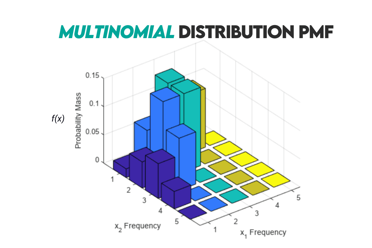
P(X\geq2) = P(X = 2) + P(X = 3) = 0.175 + 0.0083 = 0.1833 = 18.33\%

Multinomial Distribution

Definition: This distribution describes the probabilities of observing counts among multiple categories. It is a generalization of the binomial distribution.

Formulas: In essence, the PMF formula calculates the probability of a specific combination of outcomes by multiplying the number of ways that combination can occur (the coefficient) by the probability of that combination.

P(X_1 = x_1, X_2 = x_2, ..., X_k =x_k) =\frac{n!}{x_1!x_2! ... x_k!}p_1^{x_1}p_2^{x_2} ... p_k^{x_k}

Xi = the random variable representing the number of times outcome i occurs
xi = a specific value of Xi, i.e., the number of times outcome i is observed
n = the total number of trials
pi = the probability of outcome i occurring in a single trial
k = the number of possible outcomes

The sum of all xi values is equal to n:

\Sigma_{i=1}^{k}x_i = n

The sum of all pi values is equal to 1:

\sum_{i=1}^{k}p_i = 1

The coefficient represents the number of ways the observed outcomes can be arranged.

\frac{n!}{x_1!x_2! ... x_k!}

If you have two categories and observe 2 successes in the first category and 3 in the second, there are the following ways to arrange these successes:

\frac{5!}{2!3!}

The product represents the probability of observing the specific combination of outcomes.

p_1^{x_1}p_2^{x_2} ... p_k^{x_k}

There’s no separate CDF formula, as it involves summing probabilities for multiple combinations of outcomes. It’s typically computed numerically, ideally using Python, since you’re a data scientist.

The expected value for this distribution is:

E(X_i) = n*p_i

Curve: Here’s how the multinomial distribution can be visualized.

Example: Let’s say you roll a fair six-sided die 10 times. What is the probability of rolling two 1s, three 2s, one 3, zero 4s, three 5s, and one 6?

From the question, we know that

n = 10 = total\ rolls

and

p_1 = p_2 = p_3 = p_4 = p_5 = p_6 = \frac{1}{6}

To answer the question, we’ll use the multinomial distribution formula. The probability of rolling all those values from the question is 0.0834%.

P(X_1 = 2, X_2 = 3, X_3 = 1, X_4 = 0, X_5 = 3, X_6 =1) =\frac{n!}{x_1!x_2! ... x_k!}p_1^{x_1}p_2^{x_2} ... p_k^{x_k} \\ \ \\ = \frac{10!}{2!3!1!0!3!1!}*\left(\frac{1}{6}\right)^2*\left(\frac{1}{6}\right)^3*\left(\frac{1}{6}\right)^1*\left(\frac{1}{6}\right)^0*\left(\frac{1}{6}\right)^3*\left(\frac{1}{6}\right)^1 \\ \ \\ = 50,400 * \frac{1}{36} * \frac{1}{216} * \frac{1}{6} * 1 * \frac{1}{216} *\frac{1}{6} \\ \ \\ = 0.000834 \\ \ \\ = 0.0834\%

Continuous Probability Distribution

This type of probability distribution describes the probabilities of the possible values of a continuous random variable. A continuous random variable is a random variable that has an infinite number of possible values. These possible values can be associated with measurements on a continuous scale without gaps or interruptions.

Important distribution concepts:

PDF: Instead of PMF, the continuous probability distributions use the Probability Density Function (PDF). It describes the likelihood of a continuous random variable taking on a specific value or falling within a range of values.

All other concepts we’ll mention are the same as for the discrete probability distributions.

Normal (Gaussian) Distribution

Definition: It’s a distribution that has a bell-shaped probability density function, i.e., the Gaussian function. It is symmetric about its mean and is characterized by its mean (µ) and standard deviation (σ).

Formulas: Here’s the formula for the probability density function (PDF) of the Gaussian distribution.

f(x) = \frac{1}{\sigma\sqrt{2\pi}}e^{-\frac{1}{2}(\frac{x-\mu}{\sigma})^2}

f(x) = the value of the PDF at the point x
μ = the mean of the distribution
σ = the standard deviation
e = the base of the natural logarithm approximately equal to 2.71828

Any normal distribution can be converted into a standard normal distribution. It’s a distribution where μ = 0 and σ = 1. We use the following formula for the conversion:

z = \frac{x-\mu}{\sigma}

z = shows how many standard deviations x is away from the mean

The CDF for the normal distribution is given by this formula.

F(x) = P(X = x) = \frac{1}{2}\left [1 + erf\cdot \left (\frac{x - \mu}{\sigma\sqrt 2}\right)\right]

erf = the error function; you can read more about it here

The expected value is equal to the distribution’s mean.

E(X) = \mu

The same is true for the median.

\tilde x = \mu

Curve: Here’s the Gaussian distribution curve.

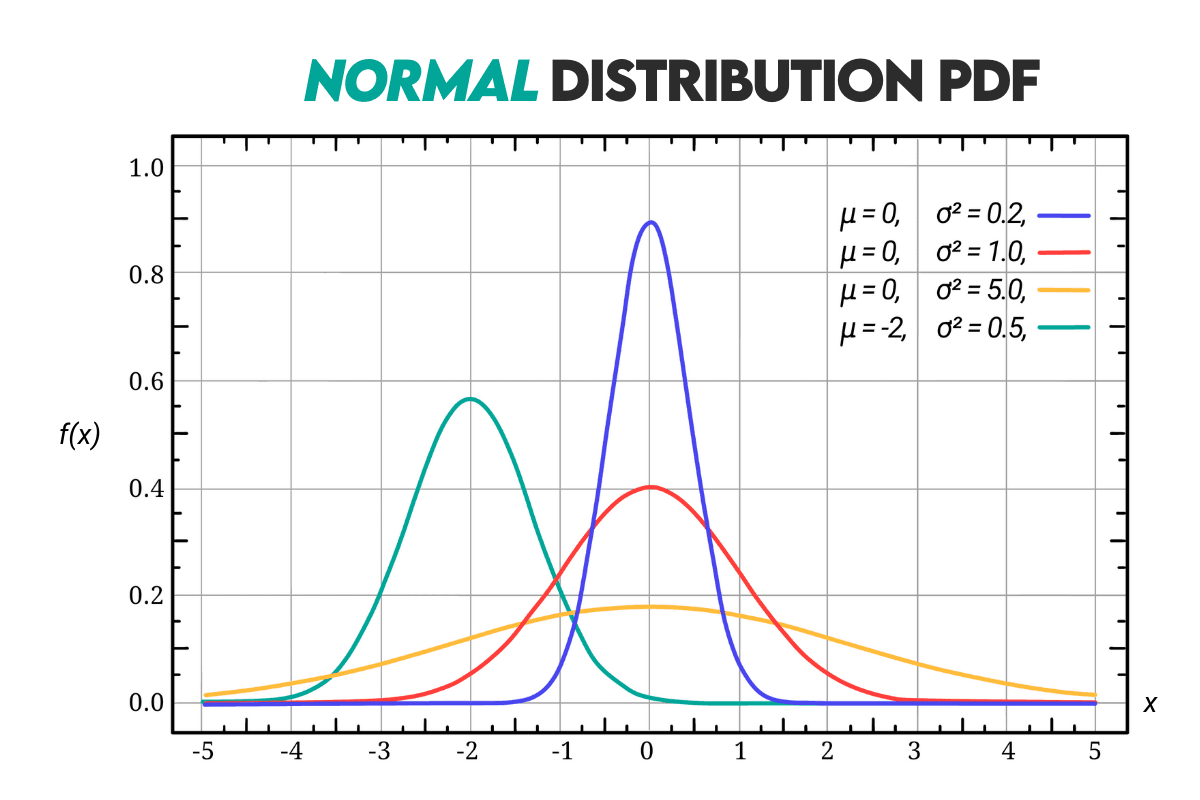
Normal (Gaussian) Distribution in Probability Cheat Sheet

Example: Here’s how you can use the z-score to calculate the probability.

Let’s say you’re looking at the students' grades on their final exam. The exam scores closely follow a normal distribution with μ = 80 and σ = 10.

What is the probability that a randomly selected student scored between 70 and 85 on the exam?

First, let’s find z for both values.

z_1 = \frac{70-80}{10} = -\frac{10}{10} = -1

z_2 = \frac{85-80}{10} = \frac{5}{10} = \frac{1}{2} = 0.5

Now we calculate the probability that a student scored between 70 and 85.

P(-1 < z\leq 0.5) = CDF(z\leq 0.5) - CDF(z\ < -1)

We will calculate it manually by looking at the z-score table, which gives us the CDF values at a particular z-score. However, the easiest way is to use the calculation software, of course.

P(-1 < z\leq 0.5) = 0.69146 - 0.15866 = 0.5328 = 53.28\%

This means there’s a 53.28% probability that the student has between 70 and 85 points on the exam.

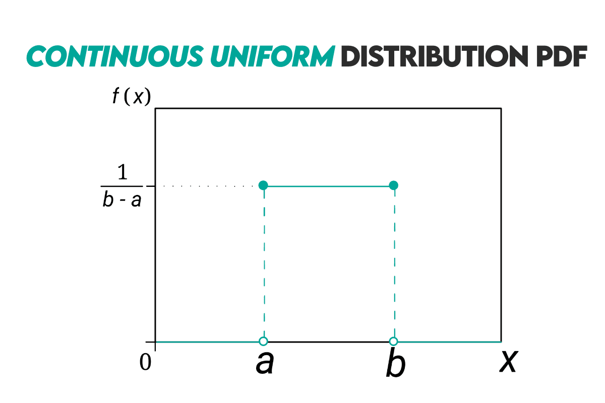
Continuous Uniform Distribution

Definition: It’s a distribution where all values within a particular interval are equally likely to occur, i.e., every data point in the interval has the same probability of occurring. It’s also known as the rectangular distribution.

Formulas: The PDF of a continuous uniform distribution is defined like this.

f(x) = \begin{cases}\frac{1}{b-a}\quad &\text {for}\ a\leq x \leq b \\ \ \\ 0\quad &\text {otherwise}\end{cases}

f(x) = the probability density at point x
a = the lower bound of the interval
b = the upper bound of the interval

To calculate CDF, use this formula.

F(x) = P(X =x) = \begin{cases} 0, & \text{if}\ x<a\\ \frac{x-a}{b-a}, & \text{if}\ a\leq x\leq b\\ 1, & \text{if}\ x>b \end{cases}

The expected value is:

E(X) = \mu = \frac{a+b}{2}

The median formula is the same:

\tilde x = \mu = \frac{a+b}{2}

Curve: Here’s how the continuous uniform distribution looks.

Continuous Uniform Distribution in Probability Cheat Sheet

Example: Let’s look at the example of a restaurant. You’re looking at the period from 6 PM to 8 PM.

You want to calculate the probability of a customer arriving at any minute in this period. So the upper bound is 8 PM, and the lower bound is 6 PM. Using the uniform distribution formula:

f(x) = \frac{1}{8:00-6:00} = \frac{1}{2\ hours} = \frac{1}{120\ minutes} = 0.0083 = 0.83\%\ per\ minute

This means that, in that period, every minute there’s a 0.83% chance that the customer will walk in.

Let’s now see the probability that the customer will walk in between 6:30 PM and 7:15 PM.

P(6:30\leq X\leq 7:15) = \frac{d-c}{b-a} \\ \ \\ = \frac{7:15-6:30}{8:00-6:00} \\ \ \\ = \frac{45\ minutes}{2\ hours}\\ \ \\ = \frac{45\ minutes}{120\ minutes} \\ \ \\ = \frac{3}{8} \\ \ \\ = 0.375 \\ \ \\ = 37.5\%

So, the probability that the guess comes between 6:30 PM and 7:15 PM is 37.5%.

Log-Normal Distribution

Definition: A distribution used to model random variables whose natural logarithms follow a normal distribution. If you take the logarithm of a variable following a log-normal distribution, the resulting values will follow a normal (Gaussian) distribution.

Formulas: The PDF function of the log-normal distribution is given as follows.

f(x) = \frac{1}{x\sigma\sqrt{2\pi}}\exp\left(-\frac{(ln(x) - \mu)^2}{2\sigma^2}\right)

f(x) = the probability density at x
x = a random variable
μ = the mean of the natural logarithm of x
σ = the standard deviation of the natural logarithm x

The CDF of the log-normal distribution is the same as the normal distribution’s.

F(x) = P(X = x) = \frac{1}{2}\left [1 + erf\cdot \left (\frac{ln(x) - \mu}{\sigma\sqrt 2}\right)\right]

And to calculate the probability of a value falling into an interval use this formula.

The expected value formula is:

E(X) = e^{\mu + \frac{\sigma^2}{2}}

The median formula is:

\tilde x = e^{\mu}

Curve: The log-normal distribution’s curve is given below.

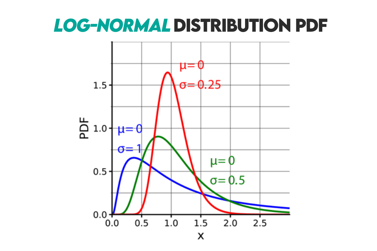
Log-Normal Distribution in Probability Cheat Sheet

Example: One of the real-life uses of the log-normal distribution is modeling income distribution. You can use it for that purpose because the personal income distribution often follows a log-normal distribution.

Let’s suppose that our parameters are μ = 10 and σ = 1.5. Now, we’ll calculate the probability that an individual's income falls between $20,000 and $40,000.

P(20,000 \leq X\leq 40,000) = CDF (40,000) - CDF(20,000) = \\ \ \\ = \frac{1}{2}\left [1 + erf\cdot \left (\frac{ln(40000) - 10}{1.5\sqrt 2}\right)\right] - \frac{1}{2}\left [1 + erf\cdot \left (\frac{ln(20000) - 10}{1.5\sqrt 2}\right)\right] = \\ \ \\ = 0.6546 - 0.4743 = 0.1803 = 18.03\%

The result shows there’s 18.03% probability that the randomly selected individual’s income is between $20,000 and $40,000.

Exponential Distribution

Definition: It’s a distribution that describes the time between events in a Poisson process, where events occur continuously and independently at a constant average rate. It is usually used to model the time until the event.

Formulas: The probability density function of the exponential distribution is given below.

f(x;\ \lambda) = \lambda e^{-\lambda x}

f(x; λ) = the probability density at value x
λ = the rate parameter, i.e., the average number of events per unit of time

The cumulative distribution function of the exponential distribution is:

F(x) = P(X =x) = 1 - e^{-\lambda x}

The expected value of the exponential function is:

E(X) = \mu = \frac{1}{\lambda}

The median for the exponential function is calculated like this.

\tilde x = \frac{ln(2)}{\lambda}

Curve: Here’s the distribution’s curve.

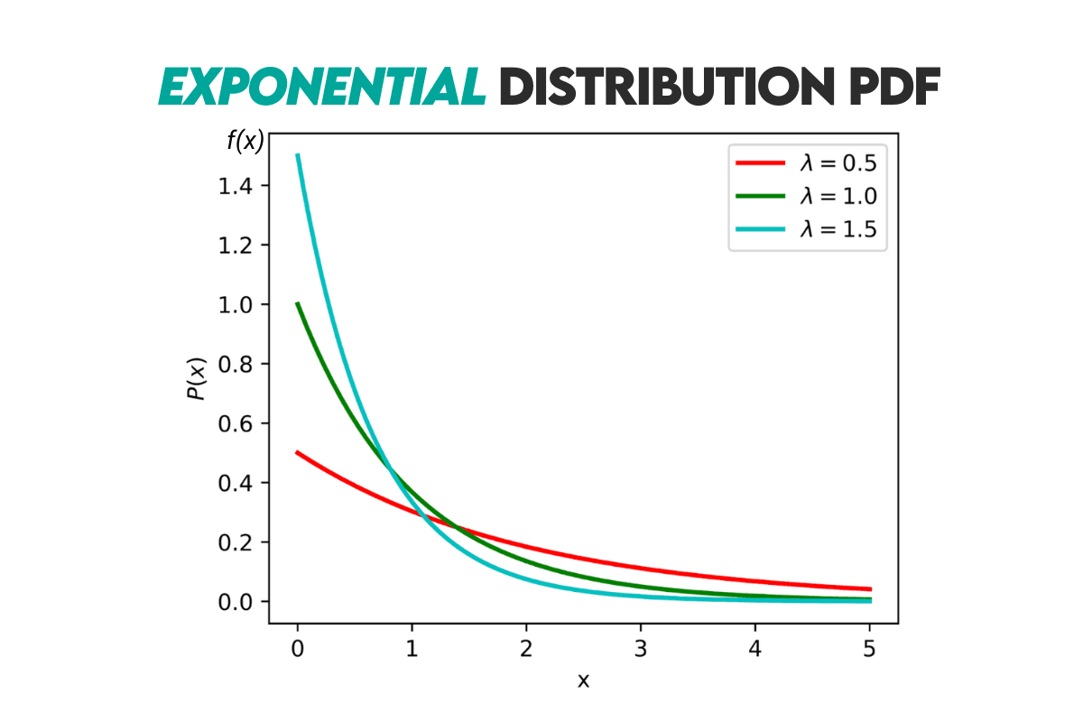
Exponential Distribution in Probability Cheat Sheet

Example: If the customers arrive at a bar at an average rate of four customers per hour, what is the probability that the next customer will arrive within 15 minutes?

We can use the CDF formula where our x is 15 minutes or 0.25 hours.

P (X \leq 0.25) = 1 - e^{-4*0.25} = 1 - 2.718282^{-1} = 1 - 0.3679 = 0.6321 = 63.21\%

The probability that the customer comes into a bar in the next 15 minutes is 63.21%.

Chi-Squared Distribution

Definition: It’s a distribution of k degrees of freedom describing the distribution of a sum of squared random variables. The chi-squared distribution can be found in statistical inference, especially in hypothesis testing and confidence interval estimation.

Formula: The probability density function of this distribution is calculated like this.

f(x;\ k) = \frac{1}{2^{\frac{k}{2}}\cdot \Gamma\left( \frac{k}{2}\right)}\cdot x^{\left(\frac{k}{2}-1\right)}\cdot e^{-\frac{x}{2}}

f(x; k) = the probability density at value x
k = the degrees of freedom which must be a positive integer
Γ(k2) = the gamma function evaluated at (k2)

The cumulative distribution function formula looks like this.

F(x; \ k) = \frac{\gamma(\frac{k}{2}, \frac{x}{2})}{\Gamma(\frac{k}{2})}

The expected values is equal to the degrees of freedom, or:

E(X) = k

The median is approximated using the following formula.

\tilde x \approx k(1-\frac{2}{9k})^3

Curve: Here’s the curve.

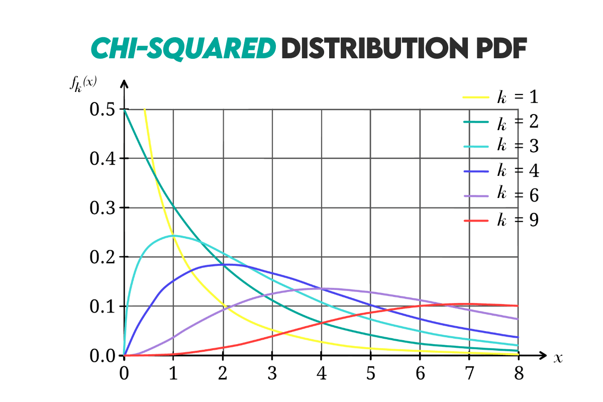
Chi-Squared Distribution in Probability Cheat Sheet

Example: Let’s say a chi-squared distribution where the degrees of freedom is 4. What is the probability that the random variable falls between 3 and 8?

Again, we need to subtract one CDF from another to calculate that.

P(a < X\leq b) = CDF_{\chi^2}(8;\ 4) - CDF_{\chi^2}(8;\ 3)\\ \ \\ = \frac{\gamma(\frac{4}{2},\ \frac{8}{2})}{\Gamma(\frac{4}{2})} - \frac{\gamma(\frac{4}{2},\ \frac{3}{2})}{\Gamma(\frac{4}{2})}\\ \ \\ = \frac{\gamma(2,\ 4)}{\Gamma(2)} - \frac{\gamma(2,\ 1.5)}{\Gamma(2)} \\ \ \\ = \frac{0.9804}{1} - \frac{0.4422}{1} \\ \ \\ = 0.4662 \\ \ \\ = 46.62\%

The result show there’s a possibility of 46.62% that the random variable will fall between 3 and 8 with the degrees of freedom equalling 4.

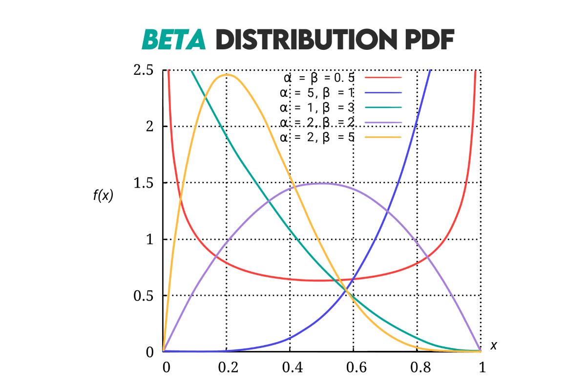
Beta Distribution

Answer: A continuous probability distribution defined by the finite interval [0, 1]. It is used in Bayesian statistics (as a prior distribution), binomial proportions (success-failure trials), quality control, A/B testing, etc.

It’s a flexible distribution and can take various shapes, from symmetric and skewed to U-shaped, depending on the values of the shape parameters α and β.

Formulas: The probability density function (PDF) of the beta distribution is given by the following formula.

f(x;\ \alpha ,\ \beta) = \frac{1}{B(\alpha,\ \beta)}\cdot x^{\alpha -1}\cdot (1-x)^{\beta -1}

x = the random variable that takes values between 0 and 1
α, β = shape parameters greater than 0
B(α, β) = the beta function; a normalizing constant that ensures the PDF integrates to 1 over the interval [0, 1]

The beta function is defined as:

B(\alpha,\ \beta) = \frac{\Gamma (\alpha)\cdot \Gamma (\beta)}{\Gamma (\alpha + \beta)}

Γ = the Gamma function

You can learn more here about the gamma function and its calculation.

The cumulative distribution function (CDF) is given by this formula.

F_X(x) = P(X = x) = \frac{B(x;\ \alpha ,\ \beta)}{B(\alpha ,\ \beta)}

The expected value of the beta distribution is given by this formula.

E(X;\ \alpha ,\ \beta) = \mu = \frac{\alpha}{\alpha + \beta}

The median is approximated using this formula.

\tilde x \approx \frac{\alpha - \frac{1}{3}}{\alpha + \beta - \frac{2}{3}}\quad \text {for}\ \alpha,\ \beta > 1

Curve: Here’s the beta distribution’s curve.

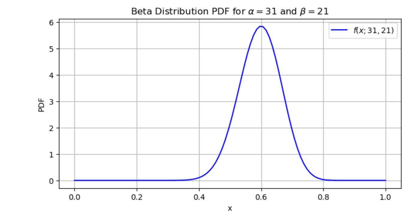
Beta Distribution in Probability Cheat Sheet

Example: We are testing the efficacy of a new medicine. We conducted a clinical trial, which showed that out of 50 patients treated with the medicine, 30 have shown a positive response. Let’s model the probability of success in this trial using a beta distribution.

From this example, we know that α = 31 (number of successful outcomes + 1), and that β =21 (number of unsuccessful trials + 1).

Let’s plot the beta distribution by calculating PDF for the values x = 0.1, 0.2, …, 0.9. We’ll do the first calculation manually, let’s say for x = 0.5, just to show you how to use the formula.

f(0.5;\ 31 ,\ 21) = \frac{1}{B(31,\ 21)}\cdot 0.5^{31 -1}\cdot (1-0.5)^{21 -1} = 2.1348166

Now, to do this manually for each point between 0 and 1 would be too much for this article. Luckily, we can use calculation tools, such as Python.

Here’s the code we used to plot the beta distribution.

import numpy as np
import matplotlib.pyplot as plt
from scipy.special import beta as beta_function

# Values of x
x_values = np.linspace(0, 1, 100)

# Shape parameters
alpha = 31
beta = 21

# Calculate the PDF for each value of x
pdf_values = (1 / beta_function(alpha, beta)) * x_values**(alpha - 1) * (1 - x_values)**(beta - 1)

# Plot the PDF
plt.figure(figsize=(8, 4))
plt.plot(x_values, pdf_values, label=r'$f(x;31,21)$', color='blue')
plt.xlabel('x')
plt.ylabel('PDF')
plt.title('Beta Distribution PDF for $\\alpha=31$ and $\\beta=21$')
plt.grid(True)
plt.legend()
plt.show()

And our plot is showing, colloquially said, the probability distribution of probabilities. The distribution shape peaks at 0.6, which means that our modeling assumptions are centered around a success rate of approximately 60%.

Gamma Distribution

Definition: It’s a distribution used for modeling the time until an event occurs. It’s used to model right-skewed distribution in fields such as reliability engineering, queuing theory, and insurance because it’s similar to the exponential distribution.

Formulas: The PDF of the gamma distribution is:

f(x) = \frac{1}{\theta^k\Gamma (k)}x^{(k-1)}e^{-\frac{x}{\theta}}

f(x; k, θ) = the probability density function
x = the random variable representing the time until the event
k = the shape parameter (a positive real number)
θ = the scale parameter (a positive real number)
Γ(k) = the gamma function, i.e., a generalized factorial function for positive real numbers

The CDF of this distribution is given by the following formula.

F(x) = P (X = x) = \frac{1}{\Gamma (k)}\gamma(k,\frac{x}{\theta})

The expected value is:

E(X) = \mu = k\theta

The median of the gamma distribution is approximated, so it’s best calculated using the calculation tools.

Curve: Here’s the distribution curve.

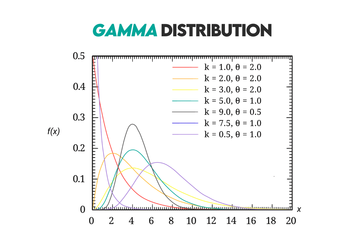
Gamma Distribution in Probability Cheat sheet

Example: You’re modeling the time until a light bulb burns out in hours. You have historical data that suggests a gamma distribution with shape parameter k = 2 and scale parameter θ = 500.

We want to answer these two questions:

1. What is the probability that a randomly selected light bulb lasts more than 600 hours?

2. What is the expected lifespan of these light bulbs?

The first question can be answered using the CDF formula.

F_X(600) = P(X > 600) \\ \ \\ = \frac{\gamma(2, \ \beta * 600)}{\Gamma(2)} \\ \ \\ = \frac{\gamma(2, \ \frac{1}{\theta} * 600)}{1}\\ \ \\ = \frac{\gamma(2, \ \frac{1}{500} * 600)}{1}\\ \ \\ = \frac{\gamma(2, \ 1.2)}{1}\\ \ \\ = 0.6626 \\ \ \\ = 66.26\%

The answer is that there’s 66.26% probability that the randomly selected light bulb will last more than 600 hours.

The second question calls for the use of the expected value formula.

E(X;\ 200,\ 500) = 2*500 = 1000\ \text {hours}

The expected lifespan of the light bulbs is 1,000 hours.

Conclusion

In this extensive cheat sheet, we focused on probability. We covered the probability main concepts, its rules, and laws. This probability cheat sheet showed you examples of the most common discrete and continuous probability distributions.

If you’re looking for more, we recommend the Statistics Cheat Sheet, which covers some other statistical concepts we didn’t touch here in this probability cheat sheet.

Don’t let it stay only on reading all this. You should practice what you have learned, and you’ll get plenty of that in our Probability and Statistics Interview Questions article.

Probability Cheat Sheet: Rules, Laws, Concepts, and Examples

Categories

What is Probability?

What Are the Rules of Probability?

1. Addition Rule

2. Rule of Complementary Events

3. Rule of Conditional Probability

4. Multiplication Rule

What Are the Laws of Probability?

Bayes’ Theorem

Law of Total Probability

Probability Distributions

Discrete Probability Distributions

Discrete Uniform Distribution

Binomial Distribution

Bernoulli Distribution

Poisson Distribution

Geometric Distribution

Negative Binomial Distribution

Hypergeometric Distribution

Multinomial Distribution

Continuous Probability Distribution

Normal (Gaussian) Distribution

Continuous Uniform Distribution

Log-Normal Distribution

Exponential Distribution

Chi-Squared Distribution

Beta Distribution

Gamma Distribution

Conclusion

Latest Posts:

Simplifying SQL Queries with Aliases: A How-To Guide

Self-Supervised Learning Guide: Super simple way to understand AI

Data Type Conversion in SQL: A Closer Look at CAST Function

Share

Follow

Categories