Probability and Statistics Interview Questions and Answers

The ultimate guide to important concepts and tips that you can apply to ace your probability and statistics data science interview questions.

Everybody knows the journey to get a data science job nowadays is tougher than ever. The immense growing popularity of data science means that we have more competition to fight for that one job. Hence, it is crucial to rightfully prepare the right things every time we get an interview.

During a data science interview preparation, most people will shift their attention more towards programming and SQL skills, or advanced concepts like deep learning, computer vision, or natural language processing. However, it’s fair to say that statistics and probability are also very important concepts to master, especially when you’re looking into a Data Analyst or Product Data Scientist role.

In this article, we are going to walk you through some important concepts and tips that you can apply to ace your probability and statistics interview questions.

The Importance of Mastering Statistics

Statistics are the heart of almost every concept that you will do as a Data Analyst or Data Scientist, it doesn't matter in which industry you’re going to work.

Imagine you’re working in an E-commerce company. To maximize the profit and customer experience, you are assigned to do a customer segmentation using one of the clustering methods. Well, the core of clustering is statistics, in which the objects which belong to the same distribution are grouped closely together.

When you’re working in a tech company and your company would like to launch a new feature or product, they will assign you to conduct an A/B test on two different products. But how do you know that one product is superior to another? Well, once again, you need to have solid statistics knowledge because we need hypothesis testing, the margin of error, confidence interval, the sample size, statistical power, and so on to judge the quality of our observations.

Also, the foundation of fancy deep learning architectures that we use for our project also come from statistics. Just take a look at Variational Autoencoders (VAE) or Bayesian Neural Networks (BNN) for example. Both VAE and BAE use a probability distribution to approximate the neural network’s parameters instead of using a deterministic value.

Having a solid knowledge of statistics makes it easier for us to understand how different deep neural network architectures work. Moreover, it is easier for us to debug problems when we implement neural networks if we know different concepts of statistics in machine learning such as overfitting, underfitting, or bias-variance trade-off.

Now that we know how important statistics is in our daily life as a Data Analyst or a Data Scientist, let’s take a look at various concepts in statistics and probability that we should prepare for our interview.

Probability Concepts You Should Know for Data Science Interview

Probability is arguably the holy grail of data science interviews. Tossing a coin, rolling a die, waiting for the bus to arrive, predicting whether it’s going to rain, you name it. There are a lot of example interview questions related to the probability that has been asked by various companies such that it’s very important for you to know exactly which concept that you should use depending on the question.

In this section, we’re going to delve into probability concepts that you should know to ace your data science interviews.

Probability Fundamentals

In this section, all of the fundamentals regarding probability concepts will be covered. As you might know, probability is the key concept of statistics and thus, it’s important that we understand the basic concept of probability.

Notations and Operations

When it comes to probability, there are going to be different notations and operations that you might encounter. These notations and operations represent specific events in the probability question that we try to solve. Different notations and operations have different meanings and of course, different solutions.

Below are the common notations and operations that you might encounter in the probability interview questions:

Union

Let’s say we have two events: A and B. The union of A and B consists of all of the outcomes from events A, B, or both.

When there is a probability question: “what is the probability that at least one event occurs?”, we always need to use a union.

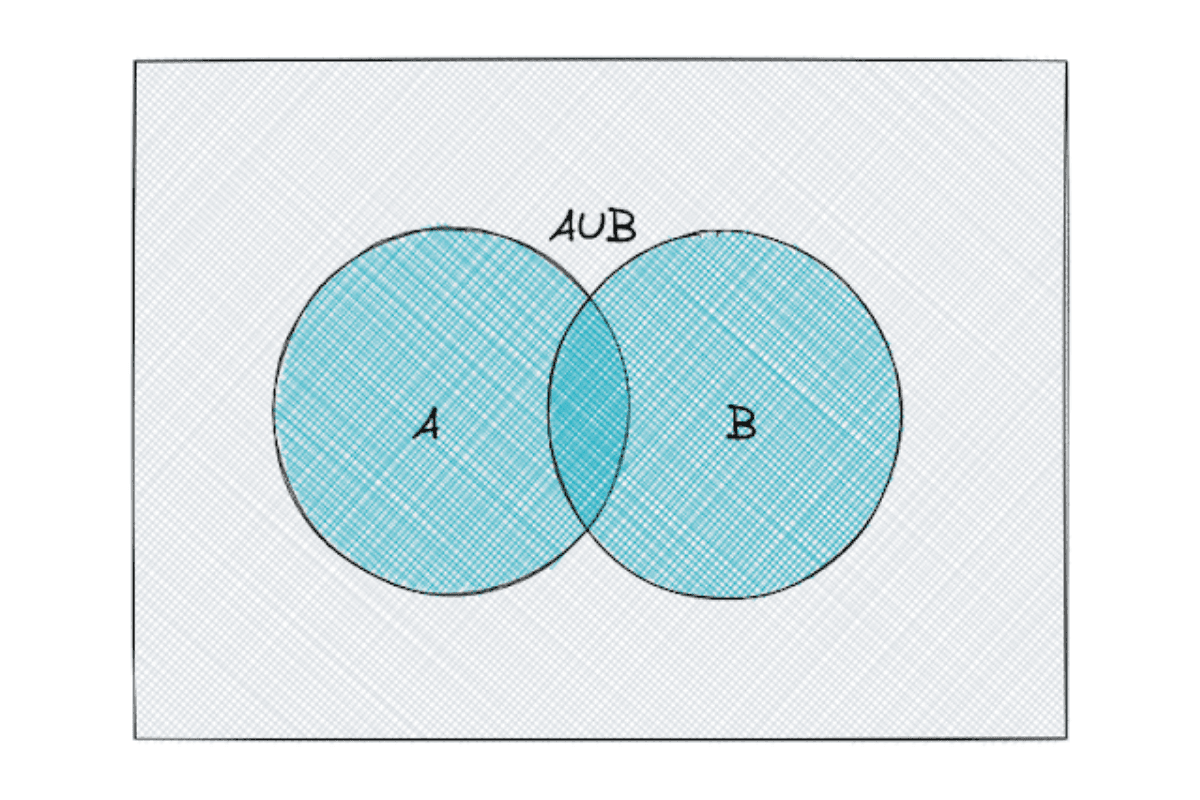
In a notation, a union of two events A and B is commonly represented as A ∪ B.

Intersection

When we have two events: A and B, the intersection of A and B consists only of the outcomes that exist in both A and B.

When there is a probability question: “what is the probability that the event A and B both occur?”, we always need to use an intersection.

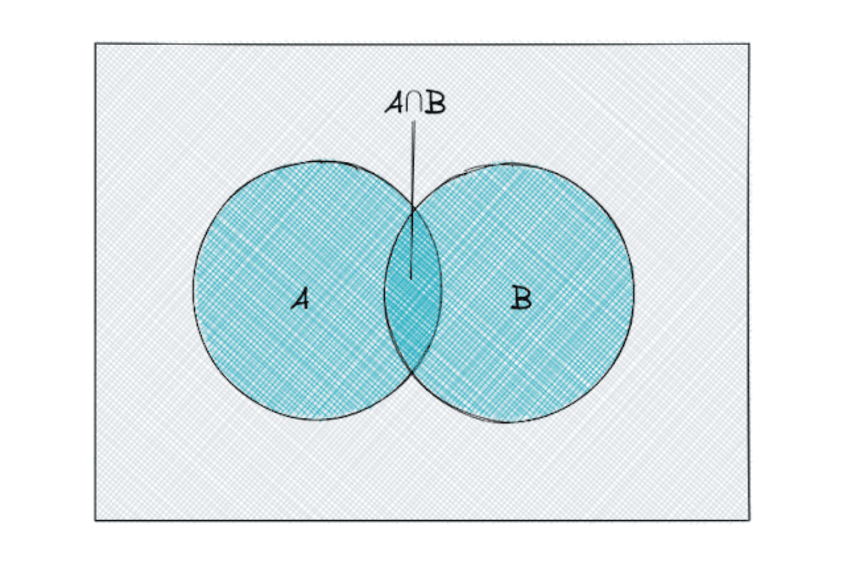
In a notation, an intersection of two events A and B is commonly represented as A ∩ B.

Mutually Exclusive

When we have two events: A and B, we can say that the two events are mutually exclusive when any of the outcomes from event A doesn’t match with any of the outcomes from event B.

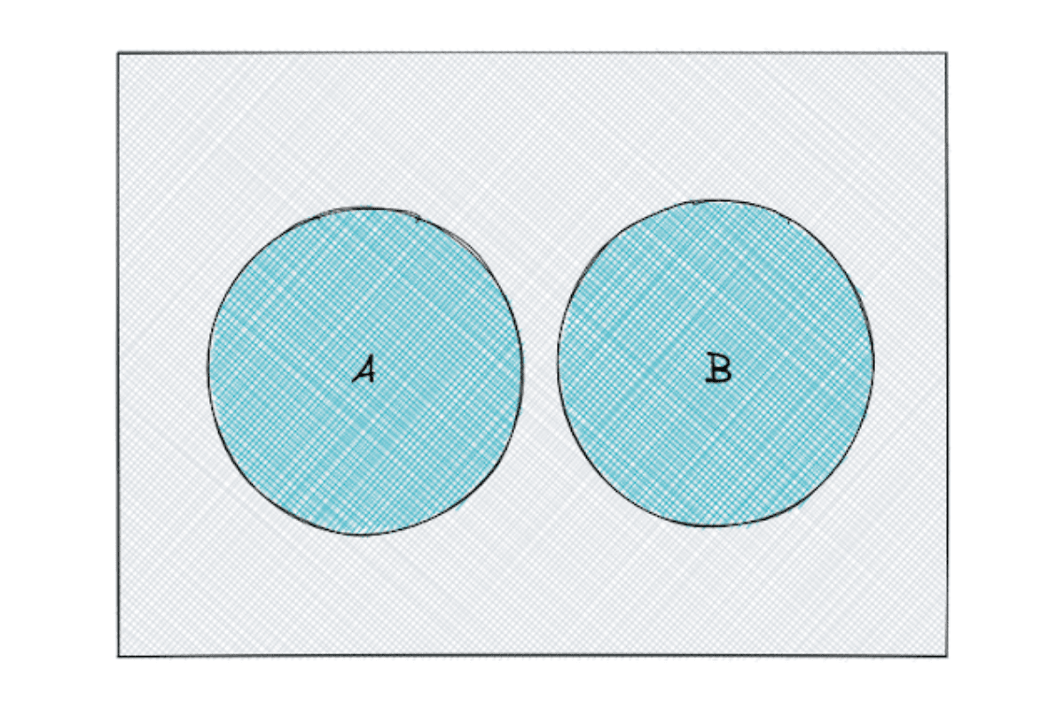
In a notation, we can say that mutually exclusive events have A∩ B = 0

Probability Properties

Probability has some important properties that we should always remember:

Probability Range

Probability always has the range between 0 to 1.

If the probability of an event is 1, this means that the event is guaranteed to happen. Likewise, if the probability of an event is 0, this means that the event is guaranteed to not happen.

The closer the probability to 1, the more likely it is that an event will occur.

In practice, the probability that an event A will occur can be denoted as P(A), where P(A) should be within the range between 0 and 1:

Probability Complements

If the probability of occurrence of an event A is P(A), then the probability of event A to not occur would be the same as:

Let’s say that we know the probability of raining tomorrow is 0.8, then the probability that tomorrow will not rain would be 1 - 0.8 = 0.2.

Probability of Union of Two Events

The probability of union of two events A and B can be defined mathematically as:

If the two events are mutually exclusive, this means that P(A∩B) = 0. Thus, the probability of union of two events in this case would be:

Example Question:

Facebook asked a question related to the probability of union of two events in one of their data science interviews. Here was the question:

“What is the probability of pulling a different color or shape card from a shuffled deck of 52 cards?”

To answer this question, first let’s define two events:

A: pulling a card with different color from a shuffled deck of cards
B: pulling a card with different shape from a shuffled deck of cards

Since there are two different colors (26 cards each) and four different shapes (13 cards each) in a deck of 52 cards, then after we pull one card out of the deck, the probability of us pulling a card with the different color would be:

Meanwhile, the probability of us pulling a card with the different shape would be:

Now, the probability of us pulling a card with different shape and color would be:

Because let’s say we get a red heart in the first pull, then the condition P(A∩B) will be fulfilled if we get a black spade or a black club in the second pull, hence in total 26 cards out of 51.

Now that we have all of the information, we can plug these values into the probability of union of two events formula:

Conditional Probability

Conditional probability is one of the probability concepts that is commonly tested in data science interviews. The good thing is, the concept of conditional probability is not difficult to comprehend.

Conditional probability can be described as the probability of occurrence of an event given that another event has occurred.

As a notation, the probability of an event A to occur given that the event B has occurred can be written as P(A|B).

Below is the formula for conditional probability.

Dependent and Independent Events

Two events can be described as dependent events if the probability of one event occurring is influencing the probability of another event occurring.

As an example, let’s say you want to draw two cards from a deck of cards and you hope to get a 5 heart in one of those draws.

At the first draw, your probability is 1/52, since there are 52 cards in a deck of cards. Now after the first draw, you notice that you didn’t get a 5 heart. In the second draw, your probability of getting a 5 heart is no longer 1/52, but 1/51. The outcome from your first draw affects your probability in the second draw. This means that the two events are dependent events.

If two events are dependent events, then the probability of the occurrence of event A given that event B has occurred is nothing different than the conditional probability:

Meanwhile, two events can be described as independent events if the probability of one event to occur doesn’t have any influence on the probability of another event to occur.

As an example, you want to toss a coin twice and you hope to get a tail in one of the tosses. In the first toss, your probability of getting a tail is ½. Now after the first toss you notice that you didn’t get a tail. However, the probability of you getting a tail in the second toss is still ½. The fact that you didn’t get a tail in the first toss doesn’t have any influence at all on your probability of getting a tail in the second toss.

If two events are independent events, then the probability of the occurrence of event A given that event B has occurred can be defined as:

because

Example Question:

Facebook asked a question related to conditional probability and dependent/independent events in one of their data science interviews. Here was the question:

“You have 2 dice. What is the probability of getting at least one 4?”

To answer this question, let’s imagine two events:

A: getting a 4 with die 1
B: getting a 4 with die 2

Since in one roll of a die we could get 6 possible outcomes, then the probability of us getting a 4 in a single roll would be ⅙. Hence:

Now the question is, what is the probability of event A and event B both to occur (P(A∩B))?

First, we need to know whether the event can be classified as a dependent or independent event. The probability of us getting a 4 with die 2 wouldn’t change regardless of the outcome of rolling die 1. Hence, we can say that our event in this question is an independent event.

Since this is an independent event, then we can say:

Next, with all of this information in hand, we can plug the values into the probability equation of union of two events:

Permutations and Combinations

Although they’re not the same, people often use the term permutations and combinations interchangeably. This is understandable since they have a very similar concept with only subtle differences. Here is the main difference between them:

In permutation, we care about the orders, while in combinations, the orders don’t matter.

So what does that mean? Let’s elaborate with an example.

Permutations

Let’s say that there is a tennis competition in our neighborhood. In total, there are 8 athletes that compete in this competition, and in the end, there are 3 medals that will be awarded.

In the first scenario, the 3 medals that will be awarded are Gold for the first winner, Silver for the second position, and Bronze for the third position. Since the medal that will be awarded is different depending on the athletes’ final positions, then in this scenario the order matters. As mentioned above, when the orders do matter, then we’re dealing with permutations.

Since we have 8 athletes:

• For the Gold medal, we have 8 possible choices: athlete 1, 2, 3, 4, 5, 6, 7, 8. Let’s say that athlete 1 wins the Gold medal.
• For the Silver medal, we have 7 possible choices: athlete 2, 3, 4, 5, 6, 7, 8. Let’s say athlete 2 wins the Silver medal.
• For the Bronze medal, we have 6 possible choices: athlete 3, 4, 5, 6, 7, 8.

Thus, we can write the scenario above as 8 x 7 x 6 = 336. This means we have 336 possible athletes’ permutations.

The general equation to solve the permutation problem is:

where n is the total number of items and k is the total number of items to be ordered.

In our example above, since we have 8 athletes, then n would be 8. Meanwhile, since we have 3 different medals to be ordered, then k would be 3. Hence:

Example Question:

Peak6 asked about the fundamental concept of permutations in one of their data science interviews. Here was the question:

“There are three people and 1st, 2nd and 3rd place at a competition, how many different combinations are there? “

Since there are three people and there are 3 places that need to be ordered and these orders are important, then we need to use the general equation of permutation.

Combinations

Let’s get back to the tennis competition example from earlier. But now instead of awarding them with Gold, Silver, and Bronze medals, we will award them with souvenirs. All of the three winners will receive the same souvenirs.

In this scenario, the order won’t matter anymore since all of the three winners receive the same souvenirs. This means that if the three winners are athletes A, B, and C, we have the following condition:

Note that the condition above doesn’t work for permutations since, in permutations, the order of the winners does matter.

The general equation for combinations is:

Same as permutations above, n is the total number of items and k is the total number of items to be ordered.

In some cases, the equation of C(n,k) above can be written as

which is the famous Binomial coefficient that you will see in the Binomial distribution in the next chapter.

Example Question:

Kabbage asked about the fundamental concept of combinations in one of their data science interviews. Here was the question:

“How to find who cheated on essay writing in a group of 200 students?”

This is the concept of combinations.

Since we have 200 students, then we have a total number of items n = 200. Next, one of the solutions to find out who’s cheating is by comparing a pair of students’ exams one by one and their order doesn’t matter, i.e a pair of student A’s and student B’s exams is the same as a pair of student B’s and student A’s exams.

Since we want to compare the exam on a pair basis, then the total number of items to be ordered k is 2. Hence we have:

Probability Distributions

Before tossing a fair coin, we know that we can only get 1 out of 2 possible outcomes, whether it’s a head or a tail. Before rolling a fair die, we know that we can only get 1 out of 6 possible outcomes. Now here comes the questions:

• What is the probability of us getting a tail if we toss a coin 5 times?
• How many tails can we get if we toss a coin 100 times?
• How many dice rolls do we need before we get a 4?

All of the questions above can be answered with the help of probability distributions.

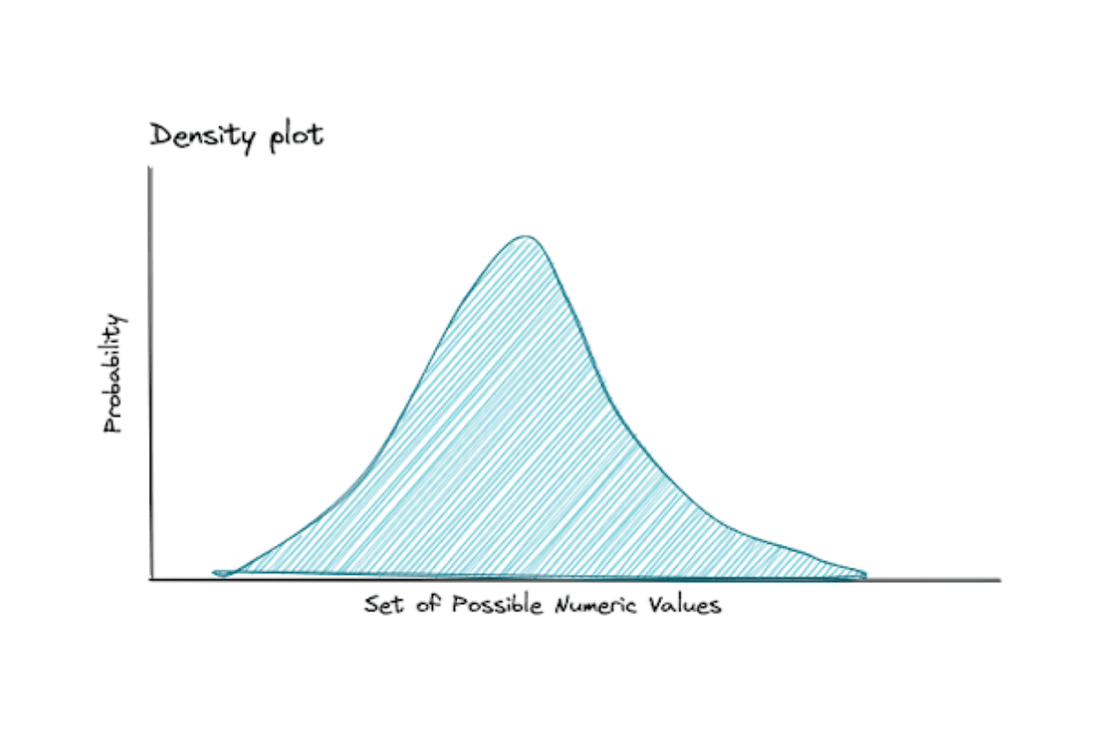
As the name suggests, probability distributions describe the probability of each outcome and they’re commonly illustrated by their probability density function (PDF) if the data is continuous or probability mass function (PMF) if the data is categorical/discrete. The x-axis describes the set of possible numerical outcomes and the y-axis describes their probabilities to appear.

There are two important properties that we can derive from probability distributions: the expected value and the variance.

• The expected value measures the average value of a sample that we expect to get if we run the trials repeatedly for the long run in a given probability distribution.
• The variance measures the theoretical limit of the variability of samples in a given distribution as the size of samples approaches infinity.

There are a lot of different kinds of probability distributions and it’s impossible to know each of them by heart. If you’re interested to learn all of the probability distributions out there, check out this link.

In this section, we’re going to guide you through some of the most commonly asked probability distributions during the interview and their use cases.

Discrete Probability Distributions

Discrete probability distribution is the type of distribution that can be used to visualize the distribution of our data if our data is categorical. This distribution is characterized by a discrete set of possible outcomes and the probability of each outcome can be modeled with the probability mass function (PMF).

The x-axis of PMF represents the possible outcomes of an event and the y-axis represents the probability of each event occurring. There are several discrete probability distributions that you should know for your data science interview preparations. Let’s start with Bernoulli distribution.

Bernoulli Distribution

Bernoulli distribution has only two possible outcomes, 0 (failure) or 1 (success) in a single trial. If the probability of success is p, then according to probability complements, the probability of failure is (1-p).

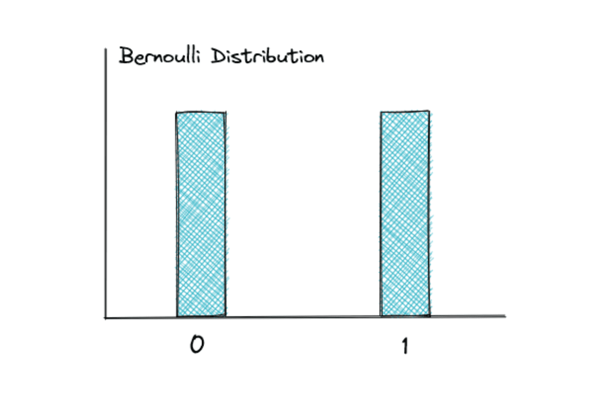
If we toss a fair coin, we know that the probability of getting a tail is 0.5. Hence, the probability of getting a head is also 0.5, as you can see in the graphic above.

However, it is important to note that the probability of two outcomes need not be equal. If we have an unfair coin, it is possible that the probability of getting a head is 0.7, while the probability of getting a tail is 0.3.

The expected value of a random variable in Bernoulli distribution is:

while the variance of a random variable with Bernoulli distribution is:

Example Question:

Facebook asked about Bernoulli distribution in one of their data science interviews. Here was the question:

“Three ants are sitting at the three corners of an equilateral triangle. Each ant randomly picks a direction and starts to move along the edge of the triangle. What is the probability that none of the ants collide?”

This is an example of a Bernoulli distribution. Three ants wouldn’t collide only if they move in the same directions, either all to the left (0) or all to the right (1). We only have 2 possible outcomes here.

Also, each ant can go in either direction and this doesn’t have any influence on another ant, hence we can classify this case as independent events.

To answer the question, we need to use the probability theory that we have discussed in the previous section.

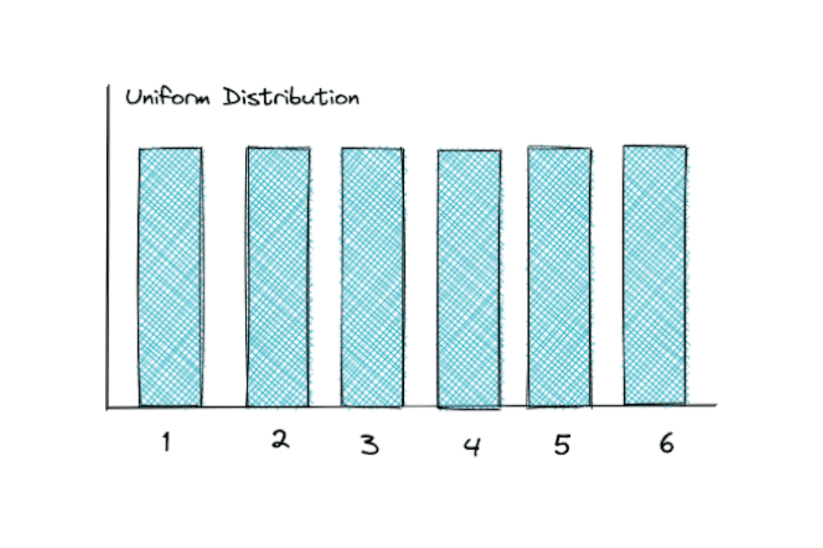
Discrete Uniform Distribution

Discrete uniform distribution can have n possible outcomes, and the probability of each outcome to occur is equally likely.

The most famous example of discrete uniform distribution is rolling a die. When you’re rolling a die, there are 6 probable outcomes that you can get, where each of them has an equal ⅙ probability. That’s why uniform distribution has a flat PMF, as you can see from the graphic below.

The expected value of a random variable in a discrete uniform distribution is:

where a is the minimum possible outcome and b is the maximum possible outcome.

The variance of a random variable in a discrete uniform distribution is:

Example Question 1:

Spotify asked about discrete uniform distribution in one of their data science interviews. Here was the question:

“Given n samples from a uniform distribution [0, d], how to estimate d?”

To answer this question, we need to take a look at the expected value of a random variable with uniform distribution. We know that the formula for expected value is:

From the question, we also know that a = 0 and b = d. Plug this information into the formula, we get:

If we have n samples, as the question mentioned, then we can estimate d with:

which is the mean of random variable X for n samples multiplied by 2.

Example Question 2:

Jane Street asked about rolling a die in one of their data science interviews:

“What is the expectation of a roll of a die?”

As you already know, rolling a die is the example of a uniform distribution.

To calculate the expectation of rolling a die, all we need to do is plug in the value into the formula of expected value:

where in our case here, a = 1 or the minimum value of possible outcome and b = 6 or the maximum value of possible outcome.

Hence, the expected value of rolling a die would be:

Binomial Distribution

The binomial distribution is an extension of Bernoulli distribution. Instead of tossing a coin once, we now toss a coin, let’s say, 100 times. Out of those 100 tosses, how many times does the coin come up tail?

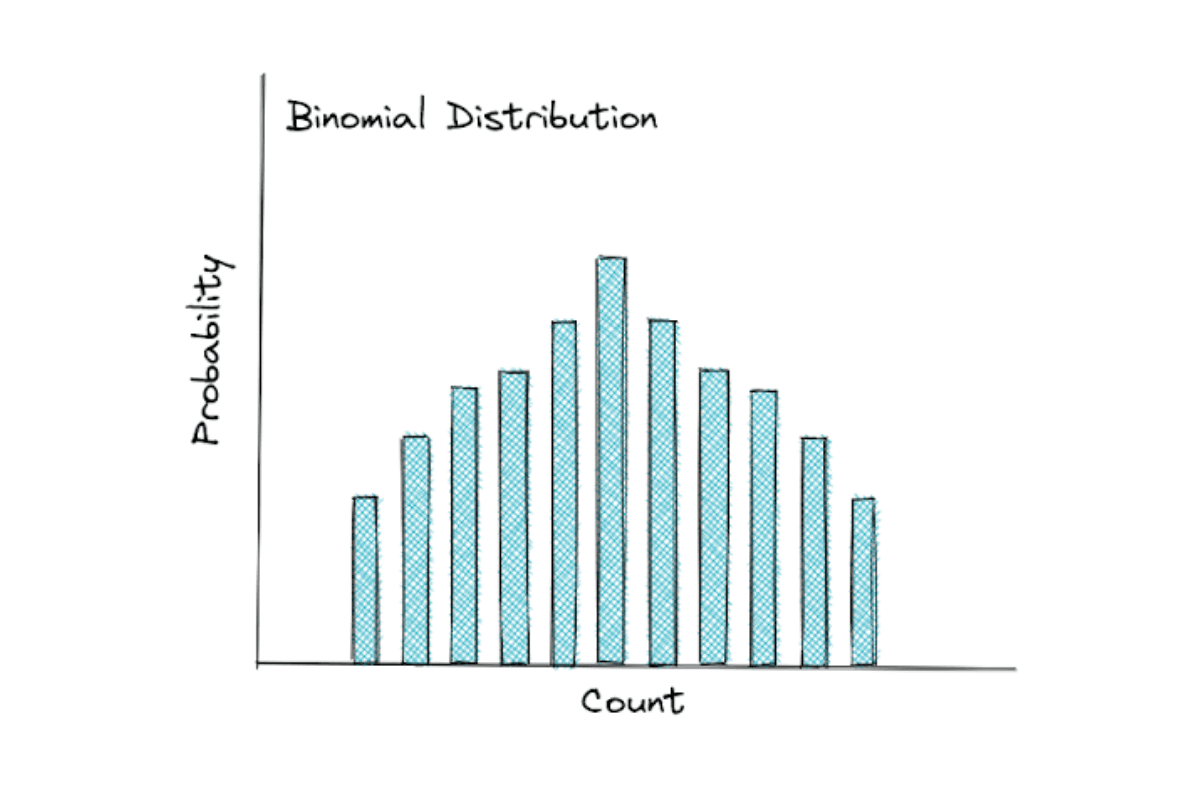
This is the example that follows a binomial distribution. It measures the probability of success in n trials. One thing to note is that each toss is independent of another, i.e the result of a coin toss doesn’t affect the probability of the result of the next toss.

The general equation of binomial distribution is as follows:

where n is the number of trials and k is the number of successes. Notice that we have a binomial coefficient there that we have discussed in the Combinations section.

The expected value of a random variable with binomial distribution is:

while the variance is:

Interview questions about binomial distribution are very common, so you definitely need to understand the concept of this distribution.

Example Question:

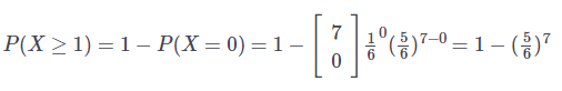
Verizon Wireless asked about binomial distribution in one of their data science interviews. Here was the question:

“What is the probability of getting at least one 5 when throwing dice 7 times?”

This question can be answered with binomial distribution by finding what is the probability of not getting any fives. In this case, the number of trials n is 7 and the number of success k is 0. Then, to get the probability of getting at least one 5, we'll need to subtract the probability of not getting any fives from 1 (total probability).

Plug this information into the equation of binomial distribution, we get:

Hypergeometric Distribution

Hypergeometric distribution is very closely related to binomial distribution above. They have more or less the same probability mass function (PMF), as you might notice below.

Let’s say we have a deck of cards and we want to draw 10 cards out of that deck sequentially. The question is, how many times will you get a heart? This use case is very similar to binomial distribution, but there is a major difference between binomial and hypergeometric distributions.

In the scenario of hypergeometric distribution, the likelihood of us getting a heart in the next draw is affected by the card that we got in the previous draw.

Before the first draw, we have a 13/52 probability of getting a heart. Now let’s say that we got a spade in the first draw, then the probability of us getting a heart in the second draw is no longer 13/52, but 13/51 since we have taken one card out from the deck. This means that each draw is not independent with another since the amount of cards in the deck will be decreased as we draw more cards.

Both binomial distribution and hypergeometric distribution measure the number of successes k in n trials. The difference is, the trials in binomial distribution are with replacement, whilst the trials in hypergeometric distribution are without replacement.

Example Question:

Facebook asked about the concept of hypergeometric distribution in one of their data science interviews. Here was the question:

“What is the probability of pulling a different color or shape card from a shuffled deck of 52 cards?”

To answer this question, let’s imagine two events:

A: probability of selecting a card with a different color

B: probability of selecting a card with a different shape

After pulling one card randomly from a shuffled deck of cards, the probability of the second card has a different color or shape (without any replacement) can be defined mathematically as:

Probability of selecting a card with a different color:

Probability of selecting a card with a different shape:

Probability of selecting a card with a different color and shape:

Thus, the probability of selecting a card with a different color or shape would be:

Geometric Distribution

Geometric distribution is also closely related with the binomial distribution. Below is the probability mass function (PMF) of geometric distribution.

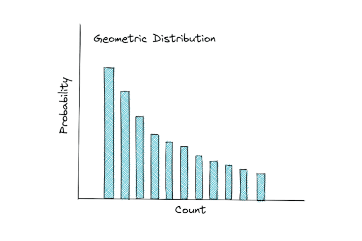
You might notice that the PMF between geometric distribution and binomial distribution are different. However, they have a very similar concept. Let’s use a coin toss as an example.

Let’s say we want to get a tail in a coin toss. With binomial distribution, we can estimate the number of tails that we will get from n coin tosses. Meanwhile with geometric distribution, we can estimate the number of coin tosses until we finally get our first tail.

Binomial distribution measures the probability of getting k successes in n trials. Geometric distribution also measures probability of success, but the number of trials itself is the outcome of it. This distribution is more interested in finding out the number of trials until we get our first success.

If the binomial distribution asks: ”how many successes in n number of trials?”, the geometric distribution asks: “how many failures until we get the first success?”. This is why the PMF of geometric distribution has the shape the way it is. The more the observations, the more unlikely it is that you didn’t get any success.

The expected value of a random variable with geometric distribution is:

where the variance can be computed as:

Example Question:

Facebook asked about the concept of geometric distribution in one of their data science interviews. Here was the question:

“You're at a casino with two dice, if you roll a 5 you win, and get paid $10. What is your expected payout? If you play until you win (however long that takes) then stop, what is your expected payout?”

To answer this question, let’s consider the following conditions:

- It costs $5 every time we want to play.
- We get $10 if we get a 5 from rolling two dice.

Our objective is that we get a 5 from rolling two dice. This means that we have 4 possibilities out of 36 different combinations: {4,1},{2,3},{3,2}, and {1,4}.

The probability of us getting a 5 from rolling two dice would be:

The expected value for a geometric distribution can be defined as:

where X is the number of trials up to and including the first success.

Since we have a probability of winning = 1/9, we can assume that we need 9 trials before we successfully get a 5. The expected payout would be:

We can model this scenario with the following equation:

Hence, the expected payout would be:

Negative Binomial Distribution

Negative Binomial distribution is basically the extension or the generalization of geometric distribution.

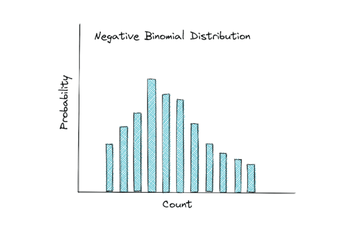
If geometric distribution asks: “how many failures until the first success?”, the negative binomial distribution asks: “how many failures until n number of successes?”. Instead of the number of failures until the first success, the negative binomial distribution extends this concept by measuring the number of failures until we reach n number of successes.

The expected value of a random variable with negative binomial distribution is:

where n is the number of successes that we’re looking for and p is the probability of success.

Meanwhile, the variance of a random variable with negative binomial distribution is:

Example Question:

Chicago Trading Company (CTC) asked about the concept of negative binomial distribution in one of their data science interviews. Here was the question:

“Toss a coin till you get 2 heads. What's the expected number of tosses to achieve this goal?”

This is an example of negative binomial distribution where we should find the number of trials up to the trials where we first found our success.

The expected value for this binomial distribution can be defined mathematically as:

where X is a coin toss that resulted in a head and n is the number of successes.

Since the coin is a fair coin, then the probability of us getting a head in a coin toss is ½ and our goal is to toss the coin until we get 2 heads (2 successes). With this information, we can plug the values into the equation above.

Hence, the expected number of tosses until we get 2 heads would be 4.

Continuous Probability Distributions

As the name suggests, continuous probability distribution is the type of distribution that can be used to visualize the distribution of our data if our data is continuous. Unlike discrete probability distributions, continuous probability distributions can’t be modeled with PMF. Instead, continuous probability distributions are modeled with the probability density function (PDF).

PDF can be defined as the area under the curve between interval A and B, as you can see from the figure below.

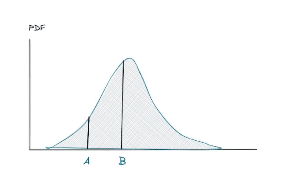
The interval between A and B can be computed with integration, but most programming language libraries or statistical software will do that for you.

Normal Distribution

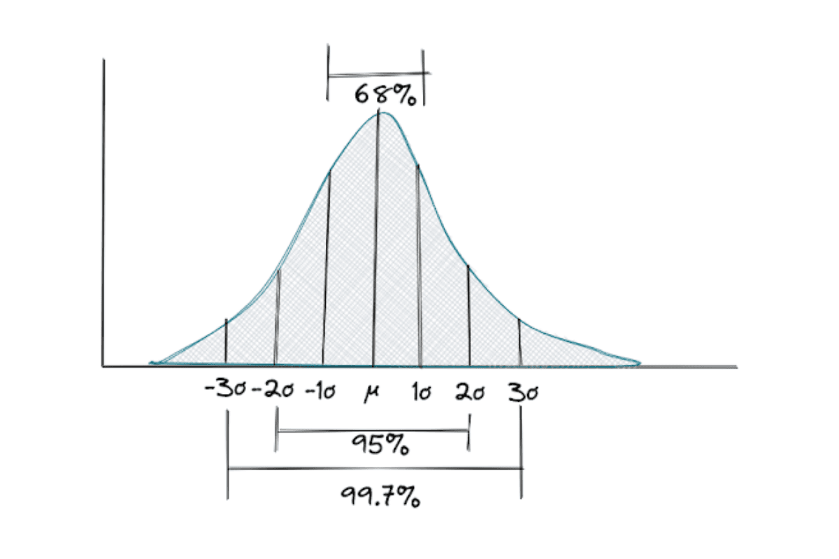
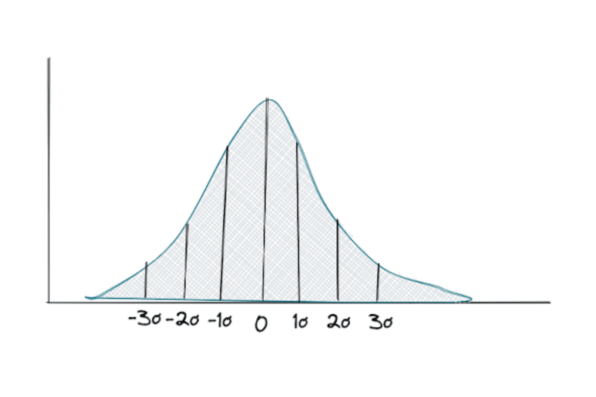
The normal distribution is the most famous distribution out there and it has a bell-curved shape as you can see in the figure above. There are two important parameters in a normal distribution: the mean and the standard deviation.

This distribution is widely used for inferential statistics due to its important properties, which is called the empirical rule.

The empirical rule is a rule that defines the normal distribution, which are:

• Roughly 68% of the observations lie within one standard deviation from the mean
• Roughly 95% of the observations lie within two standard deviations from the mean
• Roughly 99.7% of the observations lie within three standard deviations from the mean

The mean value can be any real number and non-negative and the standard deviation should also be non-negative.

Standard Normal Distribution

As the name suggests, standard normal distribution is basically a normal distribution, but with the mean value of 0 and the variance of 1. Many people also call this distribution a z-distribution, which is a distribution that people use when they want to compare the average of sample data that they have with the average of the whole population when the standard deviation of the population is known.

You will see more about the z-test and z-distribution in the statistics chapter.

Student t-distribution

The student t-distribution has a similar bell-curved shape as the standard normal distribution, but this distribution has heavier tails than the normal distribution.

The shape of this distribution will change depending on a parameter called the degree of freedom (DOF). This DOF can be defined as the sample size minus one, n-1. The larger the sample size, the more this distribution resembles the standard normal distribution.

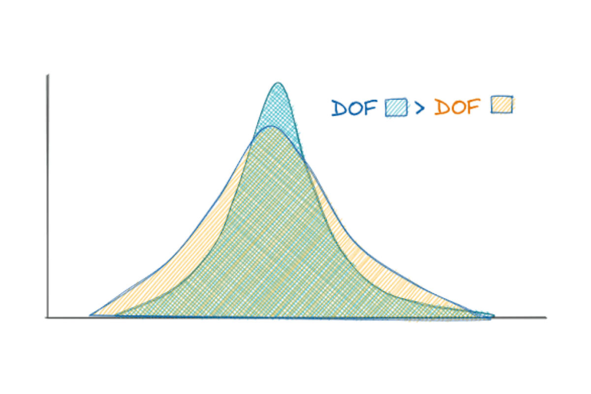
You will normally use this distribution if you want to test whether the average of your sample data corresponds to the average population when the standard deviation of the whole population is unknown.

You will see how to conduct this student t-test in the statistics chapter.

Statistical Concepts You Should Know for Data Science Interview

In this section, we have gathered all of the technical concepts regarding statistics that commonly appear in an interview that you should know: from the basic concept until the Bayes’ theorem. Let’s start from the basics.

Basic Statistics: Measures of Center (Mean, Median, Mode)

As the name suggests, mean, median, and mode measure the central tendency of data. In other words, they measure where the center of our data lies.

You might ask, if they measure the center of our data, then what’s the difference between them? It’s the method that they use to find the center of our data.

• Mean: the average of our data points
• Median: the middle point of our sorted data points
• Mode: the most frequent number in our data points

To better understand the difference between them, let’s take a look at data with different distributions as follows.

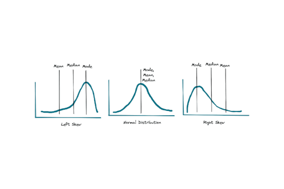
If the data is normally distributed, then the values of mean, median, and mode are all identical, as you can see in the middle image above. If the data distribution is left-skewed, then the mean will be lower than the median. Meanwhile, if the data distribution is right-skewed, then the mean will be higher than the median.

The graph above shows us one important thing: mean is a highly sensitive metric to measure the center of our data. If we have outliers in our data, the mean value could be dragged way further in comparison with the median. Thus, it’s very important to check whether outliers exist in our data before using the mean to measure the center of our data.

Example Question 1:​

Facebook asked about the concept of mean and median in one of their data science interviews. Here was the question:.

“In Mexico, if you take the mean and the median age, which one will be higher and why?”​

To answer this question, we need to find out what is the shape of age distribution in Mexico, whether it is normally distributed, right-skewed, or left-skewed.

According to Statista, it turns out that Mexico constantly has a right-skewed age distribution between 2010-2020. Hence, we can say that the mean is higher than the median.

Example Question 2:​

Although not directly related to the concept of mean, mode, and median, Airbnb asked about the following question in of their data science interviews:

“How would you impute missing information?”​

Although this question doesn’t explicitly talk about measures of the center, its concept would be very important to answer this question. Let’s say that we have numerical data and a small portion of it contains missing values. If we want to impute the missing values, we can fill them with the mean of the data or the median of the data. But which one should we choose?

We first need to check the distribution of our data and see whether outliers exist. If there are outliers, then choosing the mean to fill the missing values would introduce bias in our data and that’s not something that we want to achieve. If we have outliers in our data, using the median to fill the missing values would be the better choice as the median is more robust to outliers.

Now if we have categorical data, then it would make sense if we impute the data with the mode, which means that we fill the missing values simply with the most frequent categories that appear in our data.

Basic Statistics: Measures of Spread (Standard Deviation and Variance)

As the name suggests, measures of spread measure how spread out our data is. In general, there are 4 different metrics that we can use to measure the spread of our data: the range, the variance, the standard deviation, and the quartiles.

Range

Range is the simplest metrics to measure the spread of our data. Let’s say we have data about the annual salary of employees in a company. Let’s say that the lowest salary is $35,000 and the highest is $105,000. The range is simply the subtraction between the highest and the lowest salary. Thus the range, in this case, would be $70,000.

Variance

Variance measures the dispersion of our data around the mean. However, variance is not used frequently in a real-world application due to the fact that the values that we got from the variance were squared, i.e

where S is the variance, xi is the value of one observation, x_bar is the mean of all observations, and n is the total number of observations.

This means that the variance and the mean value have different units, e.g if the mean is in meter (m), then the variance would be in meter-square (m²). This makes variance less intuitive in terms of defining how big the spread of the data is from the mean.

Standard Deviation

Standard deviation comes to the rescue to solve the problem with variance, as it also measures the dispersion of our data around the mean. The difference is, the standard deviation is the square root of variance, i.e.

This small tweak makes the unit of observation between the mean and the standard deviation become equal, which then makes it easier for us to quantify how wide the spread of our data is around the mean.

If our data is normally distributed, i.e has a perfect bell-shaped curve, standard deviation becomes an important metric to approximate the proportion of data points in relation to their closeness to the mean.

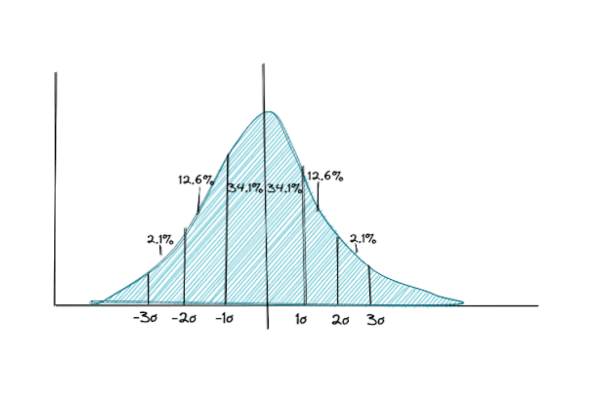
As an example, let’s say we know that the data is normally distributed and the mean annual salary of employees is $60,000. From this, we can infer that 68,2% of employees’ salaries lie in between 1 standard deviation from $60,000, around 95% between 2 standard deviations from $60,000, and 99,7% between 3 standard deviations from $60,000 (see empirical rule in the Normal Distribution section).

Quartiles

Quartiles measure the spread of our data by dividing the distribution of our data into 4 parts: the lower quartile (25% of our data), two interquartile (25%-50% and 50%-75% of our data), and the upper quartile (75% of our data). Commonly, the concept of quartiles can be easier to understand with the boxplot visualization as follows:

The questions regarding the measure of spread are very common in a data science interview, as examples, Travelport asked: “What is standard deviation? Why do we need it?” and Microsoft asked: “What is the definition of the variance?”. We have discussed the answers to both questions so far.

Example Question:​

Microsoft asked about the measure of spread concept in one of their data science interviews. Here was the question:

“How do you detect if a new observation is an outlier?”​

Although the question doesn’t explicitly mention the measures of spread, its concept is very important to answer this question. To detect an outlier, we can see where a data point lies in the distribution. If we have data that is normally distributed, then we can conclude that a data point is an outlier if it lies beyond 3 standard deviations from the mean.

We can also use a boxplot as shown above to detect if a data point is an outlier. If a data point lies above or below the maximum or minimum of a boxplot, then we can conclude that it is an outlier.

Inferential Statistics

Knowledge of inferential statistics is becoming very crucial in a data science world. This is our powerful tool to derive insight into the problem that we try to solve by observing some patterns in the data.

There are several steps and terms that you need to know within the scope of inferential statistics. Let’s start with hypothesis testing.

Hypothesis Testing

By doing hypothesis testing, you’re basically trying to test your assumptions or beliefs about the general population by looking at the sample data that you have.

This means that in hypothesis testing you would normally have:

• Null hypothesis: a hypothesis that assumes everything is fine the way it is or a skeptical hypothesis.
• Alternative hypothesis: a counter hypothesis that assumes whatever statement in the null hypothesis is not right.

As an example, you want to know whether there is a significant difference between the IQ of men and female students in a school. In this case, the hypotheses would be:

• Null hypothesis: the IQ of men and female students are the same
• Alternative hypothesis: the IQ of mean and female students are different

The main objective of hypothesis testing is to find out which hypothesis is more plausible.

However, it is important to note that the null hypothesis is always the status quo in hypothesis testing, which means that the null hypothesis is always the default true value. This means that we either reject the null hypothesis or not. This is also the reason why we never say that we ‘accept’ the null hypothesis.

Now the question is, how do we know whether or not we should reject the null hypothesis? Let’s find out in the next section.

Significance Level

The significance level is a crucial concept that we need to set during hypothesis testing. This is because the significance level will act as our tolerance before we decide to reject a null hypothesis.

The amount of significance level can vary, depending on your interest. However, the rule of thumb for significance level is 5% or 0.05.

The lower the significance level, the more cautious you’re in rejecting the null hypothesis, and vice versa.

We will elaborate further on the concept of significance level in the following sections.

Confidence Interval

The confidence interval can be described as the plausible range of values for the population parameter.

We can say that the confidence interval complements the significance level if we conduct a two-tailed hypothesis test. This means that if our significance level is 5%, then the confidence interval would be 95%, as you can see in the following figure.

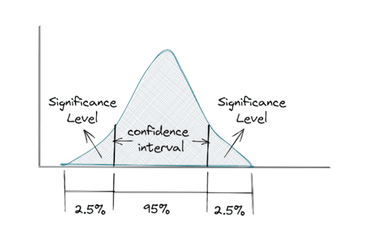
Now if your significance level is 1%, then the confidence interval would be 99%, and if your significance level is 10%, then the confidence interval would be 90%

The formula for computing the confidence interval itself can be written as:

where x_bar is the sample mean, Z is the confidence level value, σ is the standard deviation of the sample, and n is the number of samples.

The value of Z corresponds directly to your confidence interval. If the confidence interval is 95%, then Z would be 1.96.

Also, it is important to note that the equation between confidence interval value, standard deviation, and the number of observations above can be described by two different parameters: margin of error, i.e:

or the standard error, i.e:

Example Question 1:​

Tesla asked about the concept of confidence interval in one of their data science interviews. Here was the question:

“There are 100 products and 25 of them are bad. What is the confidence interval?”​

To answer this question, we need to combine our knowledge of confidence intervals with binomial distribution that we have learned in the probability section.

If there are 100 products and we know that 25 of them are bad, then we're dealing with binomial distribution in this case.

To refresh, the mean or expected value and variance of binomial distribution can be computed as follows:

where n is the total number of experiments and p is the probability of yielding a bad product.

The probability of yielding of bad product can be computed as follows:

Plug this probability value into the mean and variance equation above, we get:

Meanwhile, we know that standard deviation is the square root of variance, hence:

The standard error is the standard deviation divided by the square root of the total number of experiments.

Now we have all of the values we need to determine the confidence interval.

Example Question 2:​

Google asked about the concept of margin of error and the sample size in one of their data science interviews. Here was the question:

“For sample size n, the margin of error is 3. How many more samples do we need to bring the margin of error down to 0.3?”​

As we have seen above, the margin of error can be defined mathematically as:

From the equation above, we know that margin of error has an inverse relationship with sample size, i.e:

If the margin of error is 3 for a sample size of n, then to bring the margin of error down to 0.3, we need:

which means that we need 100*n more samples to bring the margin of error down to 0.3

p-Value

In statistics, p-Value stands for probability value. P-value represents how unlikely the result of your observation is given that the null hypothesis is true.

The lower the p-Value, the more surprising your observation is considering that the null hypothesis is true.

The combination of p-Value and significance level gives you an overview whether or not you should reject your null hypothesis in hypothesis testing.

Let’s say that the p-Value from your observation is 0.02 and your significance level is 0.05. Since the p-Value is less than the significance level, then we reject the null hypothesis in favor of the alternative hypothesis. Meanwhile, if your p-Value is 0.02 but your significance level is 0.01, then we can’t reject the null hypothesis.

Example Question:​

State Farm asked about the concept of p-Value in one of their data science interviews. Here was the question:

“What is a p-value? Would your interpretation of p-value change if you had a different (much bigger, 3 mil records for ex.) data set?”​

You can answer what a p-Value is from the definition above. Now the question is, would our interpretation of p-Value change if we had a much bigger dataset?

Our interpretation of p-Value would never change doesn't matter whether our dataset is small or big. However, if we have more data, the less the standard error would be and hence, the more robust the resulting p-Value would be.

Statistical Tests

Now we know that there are three common terminologies that we normally find in hypothesis testing: significance level, confidence interval, and the p-Value.

To choose whether we should reject the null hypothesis or not, we do statistical tests and at the end, we get the p-Value. Next, we compare the p-Value with our significance level. If the p-Value is less than the significance level, then we reject the null hypothesis in favour of the alternative hypothesis.

But how do we conduct the statistical test to get this p-Value? This is where things get a little bit tricky, since there are different statistical tests out there depending on what you want to observe. Here are the common statistical tests that you should know.

Z-Test for Population Mean

When to use this statistical test:

If we want to test if the average sample size corresponds to the average population size.

Conditions to fulfill:

• The standard deviation of the population is known
• Sample is randomly selected
• Sample is significantly smaller than population
• The variable needs to have a normal distribution

As you might already guess, the variables in this test should follow the standard normal distribution or z-distribution. In order to obtain the p-Value, we need to compute the Z value first.

Below is the formula to calculate the Z value:

where x_bar is the sample mean, μ is the population mean, σ is the standard deviation of population and n is the number of observations.

After we get the Z value, we can use the z-table or the more convenient statistical libraries in Python or R to get the corresponding p-Value.

In real-life situations, the Z-test is not performed that often because the standard deviation of the population is often unknown.

One-Sample t-Test for Population Mean

When to use this statistical test:

If we want to test if the mean of the sample data that we have corresponds to the population mean. With t-test, we have the assumption that we don’t know the population standard deviation, which is more realistic in real-life scenarios.

Conditions to fulfill:

• Sample is randomly selected
• If sample size is very small (around 15), then the data should have a normal distribution
• If the sample size is considerably large (around 40), then the test is safe to be conducted even when the data is skewed.

where x_bar is the sample mean, μ is the population mean, s is the standard deviation of the samples and n is the number of observations.

The intuition behind the t-test is similar with the Z-test, except that we don’t know the population standard deviation. Hence, we’re using the sample standard deviation.

Also, there is one additional parameter in t-test, which is the degree of freedom (DOF). The DOF is just the sample size minus 1, or n-1.

Once we know the t-value and the DOF, we can use statistical software to find the corresponding p-Value.

Paired t-Test

When to use this statistical test:

If we want to test the same sample with different treatment, and then check whether this treatment yields a statistically different result within the same sample.

The conditions to fulfill in general are the same as the one-sample t-test above. The formula to compute the t-statistic is also the same. The only difference is how we interpret the result from the t-test.

Before, the t-test measures the mean of our variable of interest. Meanwhile in this paired t-test, we are more interested in the mean or standard deviation difference of our variable of interest.

Two-Sample t-Test

When to use this statistical test:

If we want to test two different samples with different treatments, and then check whether the treatments yield a statistically different result between two samples.

Conditions to fulfill:

• Same list as the one-sample t-test
• The distribution of two samples are similar
• The result will be more reliable if the size of two samples are the same

where the index 1 and 2 denote your first and second samples, respectively.

Here the intuition of the t-statistic is the same as paired t-test, which means that the t-statistic measures the mean and standard deviation difference of our two different samples.

ANOVA (Analysis of Variance)

When to use this statistical test:

If we want to test more than two different samples with different treatments, and then check if these treatments yield a statistically different result among different samples.

The conditions to fulfill in general are the same as the two-sample t-test above, but instead of only two samples, in ANOVA there are more than two samples.

In general, below are the steps on how ANOVA is performed:

• Calculate the mean of all samples (overall mean)
• Calculate the within group deviation, which is the deviation of each member of a sample to the corresponding sample mean
• Calculate the between group variation, which is the deviation of each sample from all samples’ mean
• Calculate the F-statistic, which is the ratio of the between group variation and the within group variation

ANOVA is a time consuming test to compute by hand. Hence, you would normally conduct this test with the help of statistical software or statistical libraries in a programming language.

Check out our post 'Probability and Statistics Interview Questions and Answers' to find how you can use Python for solving Probability and Statistics questions.

Chi-Square Goodness of Fit

When to use this statistical test:

If we want to test if a sample data is a good representation of the full population. However, instead of the mean, we are looking at the proportion.

As an example, suppose we have 10 packs of M&M chocolate and there are five different colors in each pack, let’s say blue, red, yellow, green, and brown. We might want to test whether the proportion of these five colors in each pack is equal or not.

Conditions to fulfill:

• The sample is randomly selected
• Our data should be categorical or nominal. Since we are interested in proportion, then this test is not appropriate for continuous data
• The sample size is large enough such that there are at least 5 items in each data category.

Below is the formula of Chi-Square Goodness of Fit test:

where O is the observed frequency counts in each category, E is the expected frequency counts in each category, and k is the total number of categories.

After computing the Goodness of Fit, at the end we will get the p-Value, same as the other tests mentioned above that gives us the insight whether or not we should reject the null hypothesis.

Chi-Square Test of Independence

When to use this statistical test:

If we want to test if two or more sample data are likely to be related or not. The idea is similar to ANOVA.

However, if in ANOVA we are interested in the mean, in this test we are more interested in the proportion. As an example, let’s say that we own a cinema. We want to know if the genre of the movie and the amount of snacks that people buy are related. The genre of the movie is our first sample data, and the amount of snacks is our second sample data.

The conditions to fulfill are in general the same as the Goodness of Fit above, except that instead of just one sample, in this test we should have two or more samples.

Below is the formula of Chi-Square test of independence:

where r and c are the two different categories that you observe, i.e from the example above, r might be the genre of the movies and c might be the snacks.

After computing the formula above, we will get the p-Value at the end which we can use to decide whether we should reject the null hypothesis or not.

Example Question:​

In one of their data science interview, Amazon asked about a concept that put our knowledge about different statistical measures into action. Here was the question.

“In an A/B test, how can you check if assignment to the various buckets was truly random?”​

Since we have an A/B test here, then let’s say we have two variables called A and B. If the assignment is truly random, then there should be no statistically significant difference between two variables.

Now since we are interested in checking whether the assignment is truly random, then we can compare the mean of two variables if they are continuous variables. If there is only one treatment that will be applied, then we can use the two-sample t-test. Meanwhile if there are multiple treatments, then we can use ANOVA.

If we want to know whether variable A and variable B are related to each other and they are categorical variables, then we can use the Chi-Square test of independence.

Steps of Hypothesis Testing

Now we know all of the things about inferential statistics! Let’s sum it up and gather all of the necessary steps that we need to properly conduct hypothesis testing:

• First, set up the hypotheses: the null hypothesis and the alternative hypothesis
• Choose your significance level
• Conduct statistical test that suit your type of observation
• Find the p-Value from statistical test
• Make the decision whether or not to reject the null hypothesis

Example Question:​

Facebook asked about the end-to-end concept of inferential statistics in one of their data science interviews. Here was the question:

“We have a product that is getting used differently by two different groups. What is your hypothesis about why and how would you go about testing it?”​

When we have a product that is getting used by two different groups, then we need to first gather the data, and then we can analyze the result using the two-sample t-test.

1. We formulate our hypothesis as follows:

- null hypothesis: the average used rate between 2 groups are the same
- alternative hypothesis: the average used rate between the 2 groups are different.

2. We pick our significance level, usually around 0.05

3. From the data, we can get the average and the standard deviation of each group.

4. Then, we compute the t-statistics using the two-sample t-test.

5. If the resulting t-test is below our significance level (< 0.05), then we can reject our null hypothesis in favor of our alternative hypothesis, i.e the average used rate between the 2 groups is different.

6. If the resulting t-test is above our significance level (> 0.05), then we can stick with our null hypothesis, i.e the average used rate between the 2 groups is more or less the same.

Statistical Power

As you already know, when you have a p-Value after conducting a statistical test, you will have the power to decide whether or not to reject the null hypothesis by comparing it with your significance level.

However, statistical inference will always come with uncertainty. This uncertainty mainly comes from your significance level, which you can fine-tune depending on your research, as well as the sample data quality that you have gathered for a statistical test.

This means that you’re prone to making two types of error during hypothesis testing, which in statistics are commonly referred to as Type I error and Type II error.

• Type I error means that you’re falsely rejecting the null hypothesis
• Type II error means that you’re failing to reject the null hypothesis

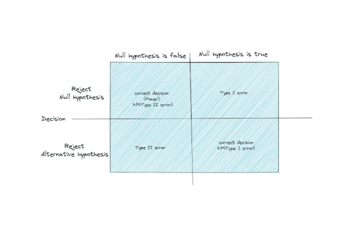
Statistical power is the probability that you’re correctly rejecting the null hypothesis. This also means the probability of making less Type II error. The higher the statistical power, the lower the probability of you making the Type II error.

Power Analysis

Now you know there are two types of error that you might encounter when conducting hypothesis testing. As mentioned before, one of the common sources of the error is the data quality. This means that you probably don’t have enough sample data to produce a p-Value that convincingly concludes whether you should or should not reject the null hypothesis.

The question that often arises in power analysis is: “What are the minimum samples required to make sure that the p-Value that we get is convincing enough for us to reject the null hypothesis?”

There are 4 parameters that normally take into account in power analysis calculations: the effect size, the sample size, the significance level, and the statistical power.

You already know the sample size, the significance level, and the statistical power from the sections above. The effect size, however, is normally calculated using statistical measures, for example Pearson’s correlation if you want to measure the relationship between variables, or Cohen’s d if you want to determine whether the difference between variables is significant.

In a power analysis, you need to define the value of effect size, significance level, and statistical power in advance to find out the required sample size.

The default value for significance level is 0.05, the default value for Cohen’s d to discover large effect size is 0.80, and the default value of statistical power is also 0.8. However, you can fine tune those values depending on your research and this requires a knowledge in the subject matters.

Power analysis is a daunting task to compute by hand, hence normally it is implemented in statistical libraries in a programming language.

Bayes’ Theorem

In the last section, we were talking about inferential statistics that are commonly used in frequentist perspective. In this section, we are going to talk about a different perspective of inferential statistics, which utilize Bayes’ theorem.

Bayes’ theorem is a statistical approach which is conducted by applying probability theory. This theorem in some sense has the same analogy as how a human infers about something in real life. It has a prior belief of the occurrence of an event, and this belief will be updated as the new evidence or data is supplied. In the end, it produces a posterior belief.

The fundamental concept behind Bayes’ theorem is commonly called Bayes’ rule. This rule is similar to what you have seen in the conditional probability section above.

Below is the equation of Bayes’ rule:

where A and B are the events.

We can define P(A|B) as the probability of the occurrence of event A given that event B has occurred. Likewise, we can define P(B|A) as the probability of the occurrence of event B given that event A has occurred.

Beside that, the Bayes’ rule above also shows the fundamental concept of this rule: prior, likelihood, marginal, and posterior, as you can see below:

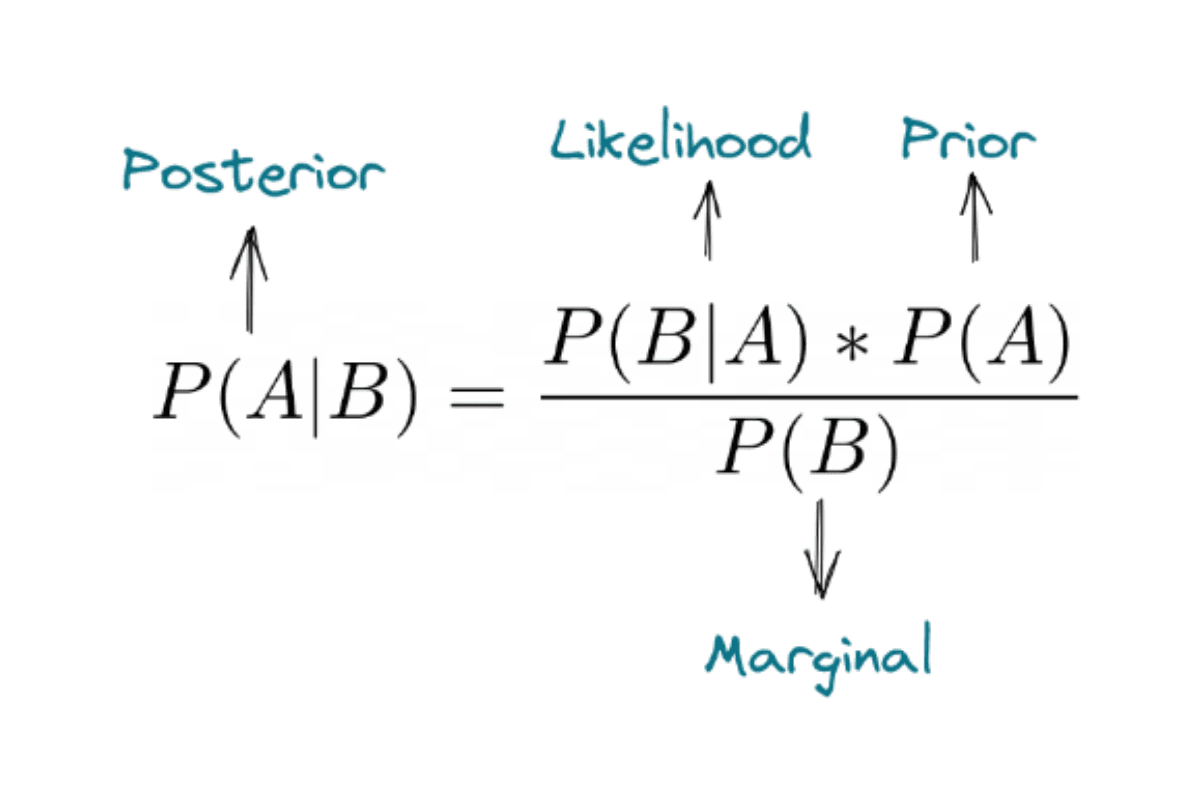
To elaborate more, here are the questions that posterior, likelihood, prior, and marginal actually try to answer:

• Posterior: how probable is our hypothesis given the observed evidence?
• Likelihood: how probable is the evidence given that our hypothesis is true?
• Prior: how probable is our hypothesis before we see any observations or evidence?
• Marginal: how probable is the evidence under all possible hypotheses?

Example Question:​

Facebook asked about the concept of Bayes’ theorem in one of their data science interviews. Here was the question:

“You're about to get on a plane to Seattle. You want to know if you should bring an umbrella. You call 3 random friends of yours who live there and ask each independently if it's raining. Each of your friends has a 2/3 chance of telling you the truth and a 1/3 chance of messing with you by lying. All 3 friends tell you that "Yes" it is raining. What is the probability that it's actually raining in Seattle?”​

To answer this question, let’s first assume a variety of events:

- A: raining in Seattle
- A’: not raining in Seattle
- Xi: random variable with Bernoulli distribution, such that
Xi = 1, if a friend says “Yes, it will be raining in Seattle”
Xi = 0, if a friend says “No, it won’t be raining in Seattle”

Now, since we don’t have any information about the probability of rain in Seattle, let’s assume it to be 0.5, hence:

In the question, it is stated that all of the three friends said “Yes, it will be raining in Seattle”. We can express this as:

We know that the probability of our friends telling the truth is ⅔.

We can express the probability of our friend told us 'Yes, it will be raining in Seattle' given that now is raining in Seattle as:

and the probability of our friend told us 'No, it won't be raining in Seattle' given that now is not raining in Seattle as:

Now that we got the information we need, we could find out the probability of raining in Seattle given that our three friends say 'Yes' with Bayes’ theorem as follows:

Tips on Preparing Probability and Statistics Interview Questions

We can agree that learning statistics, either it is for the exam or the interviews, is not easy. As you can see from the sections above, there are a lot of topics that we need to cover in order to at least have a general understanding of statistics and probability.

The tips below might be helpful for you to ace your probability and statistics interview questions.

Learn the Concepts

You learn statistics the wrong way if you’re learning the formula instead of the concepts. The thing is, you can always look back at the textbook if you forget the formula. However, if you forget the concept, then you wouldn’t be able to answer the question with the correct approach.

It is better to learn the concept because then you will be able to approach each question correctly, i.e whether we consider the problem can be solved with binomial distribution, geometric distribution, or negative binomial distribution.

As an example, when you get a question that asks what is the probability of getting 5 tails in 20 coin tosses, you should know that this question can be answered with binomial distribution. It’s fine if you forget the equation of binomial distribution because you can always look it up on the internet or textbook. The most important thing is that you know that this problem can be solved with binomial distribution.

Always learn the concepts, not the formula.

Use Pen and Paper

Let’s be real, when we’re dealing with statistics and probability questions, we’re dealing with maths. Thus, don’t try to solve probability and statistics interview questions all directly in your mind. Instead, use a traditional way like a pen and a paper to brainstorm your thoughts.

Whenever you put your thoughts on a piece of paper, then it will be easier for you to solve the problems in a step-by-step manner and you will think about the problem and how to solve it in a more concise way.

Don’t Learn Every Concept in One Sitting

Mastering statistics is like trying to gain muscles or lose your weight, it can’t happen in just one sitting or one gym session. Instead, it is built based on consistent exercises that occur within specific time periods.

Set aside about one hour each day to try to solve probability and statistics interview questions within a time period of your choice and don’t forget to take a scheduled time off as well. The most important thing is the consistency of learning.

After some time, it is guaranteed that you will get used to statistics questions and you will be able to see that there are recurring patterns in probability and statistics interview questions. You will be able to understand which concept you should apply in each question, i.e whether you should use ANOVA or Chi-Square, whether you should use geometric or hypergeometric distribution, etc.

Read or Listen to the Question Carefully

When you get probability and statistics interview questions, it is very important to make sure that you understand the problem that you’re trying to solve. But how do we make sure of that?

Here is the trick: you can paraphrase the question with your own words to the interviewee and then ask them if your paraphrase corresponds to the question being asked. This method serves you two purposes: to make sure that you understand the question correctly and also to buy you a little bit of time to think about the solution.

Always Ask for a Clarification

After understanding the question being asked, make sure to ask for any clarifications or assumptions if you feel like the question is incomplete and you need more context from the question.

This is because probability and statistics interview questions are full of assumptions that you need to take care of, i.e whether one event is independent or dependent on another, whether the data is continuous or categorical, whether we’re looking for mean or proportion in an A/B test, and so on. Only after you understand the question completely can you offer the right solution.