Machine Learning Types: Here is How to Differentiate Them

A detailed guide to understanding the various types and applications of machine learning

In a quiet lab, a computer mistakenly identified a picture of a dog as a wolf; the reason wasn't its keen algorithmic insight but the sunny background common in wolf pictures.

This simple mistake underscores the complex and nuanced world of machine learning, a field reshaping every facet of how we interact with technology.

In this one, we’ll divide Machine learning into supervised, unsupervised, and reinforcement learning. We’ll talk about other machine learning types, even if they are rare, and at the end, we’ll talk about how to select ML algorithms for your project. Let’s start.

Supervised Learning

Machine learning, called supervised learning, uses labeled data to train models. It is like teaching with examples. Inputs and the right outputs are coupled in the training data.

Key Applications and Examples

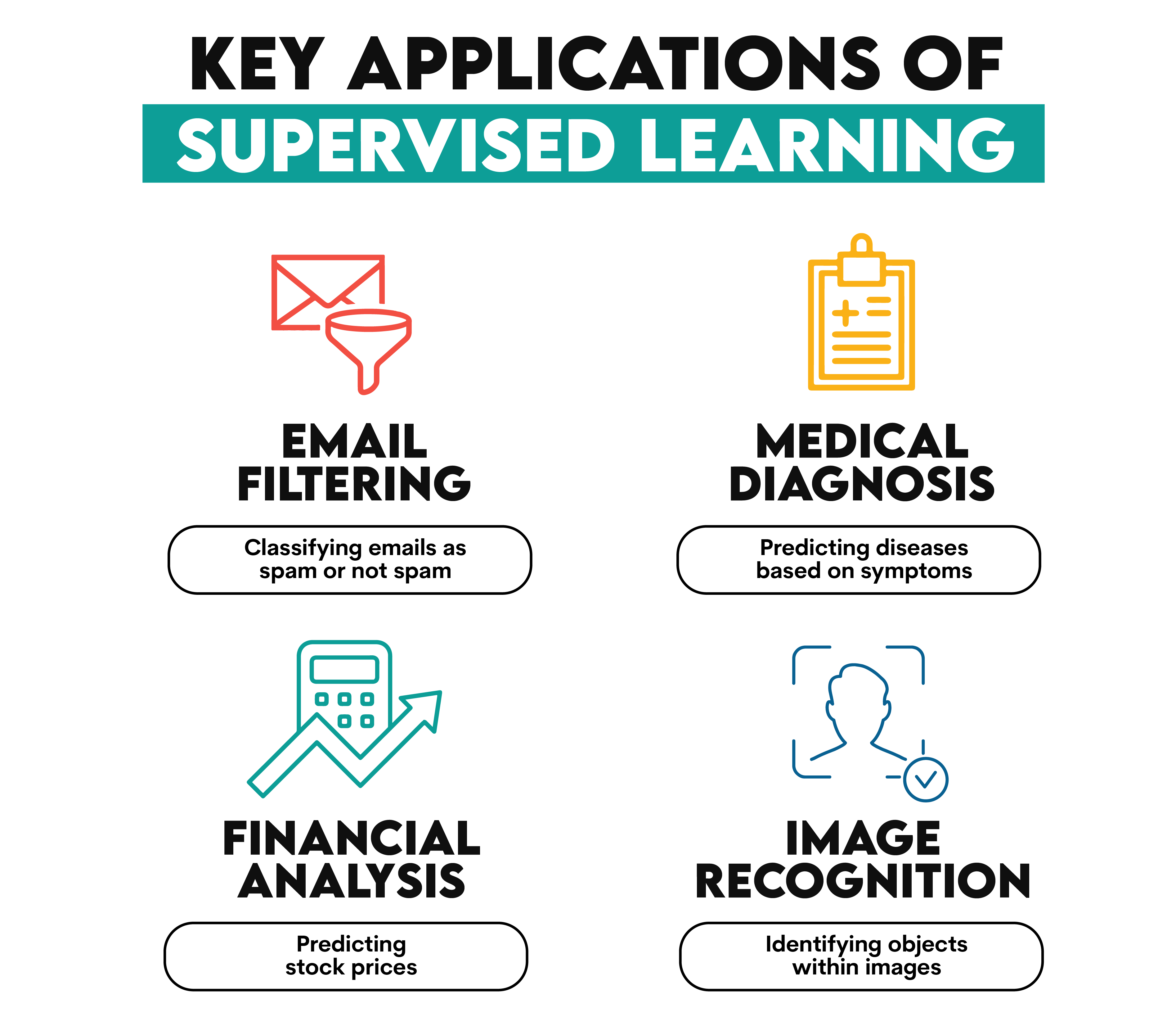
• Email filtering: Classifying emails as spam or not spam.
• Medical diagnosis: Predicting diseases based on symptoms.
• Financial analysis: Predicting stock prices.
• Image recognition: Identifying objects within images.

Advantages

Supervised Learning models have the predictive power to make accurate predictions with enough training data, and their results are usually easy to understand and interpret.

Limitations

One significant challenge with Supervised Learning is that it requires a lot of labeled data, which can be costly, time-consuming, and sometimes hard to collect.

Moreover, there's a risk of overfitting, where the model performs too well on the training data but poorly on unseen data.

Popular algorithms

Now, let’s look at the popular algorithms and their simple explanations.

• Linear Regression: Predicts a continuous output.
• Logistic Regression: Used for binary classification tasks.
• Support Vector Machines (SVM): Finds the best boundary between data points of different classes.
• Neural Networks: Can model complex patterns using layers of neurons.

Application of Supervised Learning Algorithms

Wonderful, let’s apply those algorithms above at once and evaluate them.

To do that, first, let’s load those datasets.

from sklearn.datasets import load_wine
from sklearn.preprocessing import StandardScaler
from sklearn.model_selection import train_test_split
from sklearn.linear_model import LogisticRegression, LinearRegression
from sklearn.svm import SVC
from sklearn.neural_network import MLPClassifier
from sklearn.metrics import accuracy_score, r2_score
import pandas as pd
import matplotlib.pyplot as plt

Next, let’s load the wine dataset and make it read to build those models. In the end, you’ll see how these algorithms can be applied one by one and add the evaluation metrics to the dataframe to compare them at the end.

# Load the wine dataset
wine = load_wine()
X_wine = wine.data
y_wine_quality = wine.target  # For classification
# For simplicity in regression, let's predict the total phenols (a continuous feature) from the wine dataset
# This is just for demonstration and not a standard practice
X_wine_regression = StandardScaler().fit_transform(X_wine)  # Standardize for neural network efficiency
y_wine_phenols = X_wine[:, wine.feature_names.index('total_phenols')]  # Selecting a continuous feature

# Split the dataset for classification
X_train_class, X_test_class, y_train_class, y_test_class = train_test_split(X_wine, y_wine_quality, test_size=0.2, random_state=42)

# Split the dataset for regression
X_train_reg, X_test_reg, y_train_reg, y_test_reg = train_test_split(X_wine_regression, y_wine_phenols, test_size=0.2, random_state=42)

# Reinitialize models to reset any previous training
logistic_model = LogisticRegression(max_iter=200)
svm_model = SVC(probability=True)
neural_network_model = MLPClassifier(max_iter=2000)
linear_regression_model = LinearRegression()

# Train and evaluate models for classification
logistic_model.fit(X_train_class, y_train_class)
logistic_pred_class = logistic_model.predict(X_test_class)
logistic_accuracy = accuracy_score(y_test_class, logistic_pred_class)

svm_model.fit(X_train_class, y_train_class)
svm_pred_class = svm_model.predict(X_test_class)
svm_accuracy = accuracy_score(y_test_class, svm_pred_class)

neural_network_model.fit(X_train_class, y_train_class)
neural_network_pred_class = neural_network_model.predict(X_test_class)
neural_network_accuracy = accuracy_score(y_test_class, neural_network_pred_class)

# Train and evaluate Linear Regression for regression
linear_regression_model.fit(X_train_reg, y_train_reg)
linear_regression_pred_reg = linear_regression_model.predict(X_test_reg)
linear_regression_r2 = r2_score(y_test_reg, linear_regression_pred_reg)

# Store results in a DataFrame
results_df_wine = pd.DataFrame({
    'Model': ['Logistic Regression (Class)', 'SVM (Class)', 'Neural Network (Class)', 'Linear Regression (Reg)'],
    'Accuracy/R²': [logistic_accuracy, svm_accuracy, neural_network_accuracy, linear_regression_r2]
})

# Display the DataFrame
results_df_wine

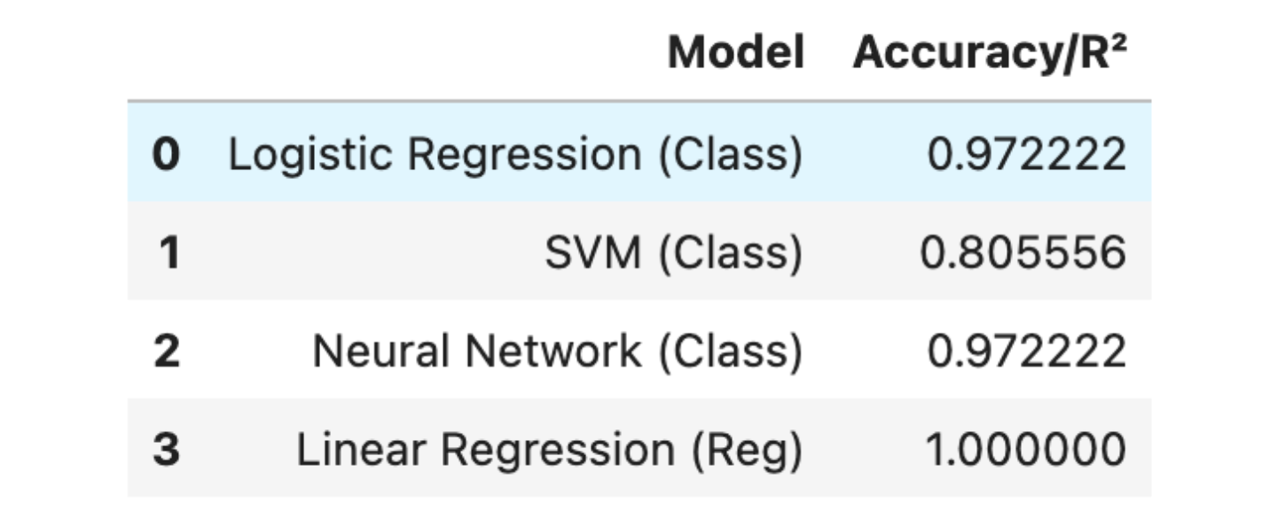
Here is the output.

Now, let’s make this output look better.

# Plotting results for the Wine dataset
plt.figure(figsize=(10, 6))
plt.barh(results_df_wine['Model'], results_df_wine['Accuracy/R²'], color=['blue', 'orange', 'green', 'red'])
plt.xlabel('Score')
plt.title('Model Evaluation on Wine Dataset (Classification & Regression)')
plt.xlim(0, 1.1)  # Extend x-axis a bit for clarity
for index, value in enumerate(results_df_wine['Accuracy/R²']):
    plt.text(value, index, f"{value:.2f}", va='center')
plt.savefig("supervised.png")
plt.show()

Here is the output.

Now, let’s evaluate the results.

• Logistic Regression: Shows excellent performance for classification with 97% accuracy, suggesting a strong fit for the dataset's pattern.
• SVM: Shows lower accuracy at 81%, indicating potential underfitting or the need for parameter tuning and kernel choice optimization.
• Neural Network: Achieves high accuracy similar to logistic regression, reflecting its capability to model complex relationships in the dataset.
• Linear Regression: Reports an unrealistic perfect R² score, implying an overly optimistic fit that warrants further scrutiny for potential data leakage or overfitting.

Unsupervised Learning

Unsupervised Learning involves training models using data that doesn't have labeled responses. That means no example data you want to predict exists in the dataset.

Using this method, the algorithm attempts to learn the data structure without being given specific predictions. It finds patterns by reducing the dimensionality of the data and grouping the data points into clusters based on similarities and differences.

Key applications and examples:

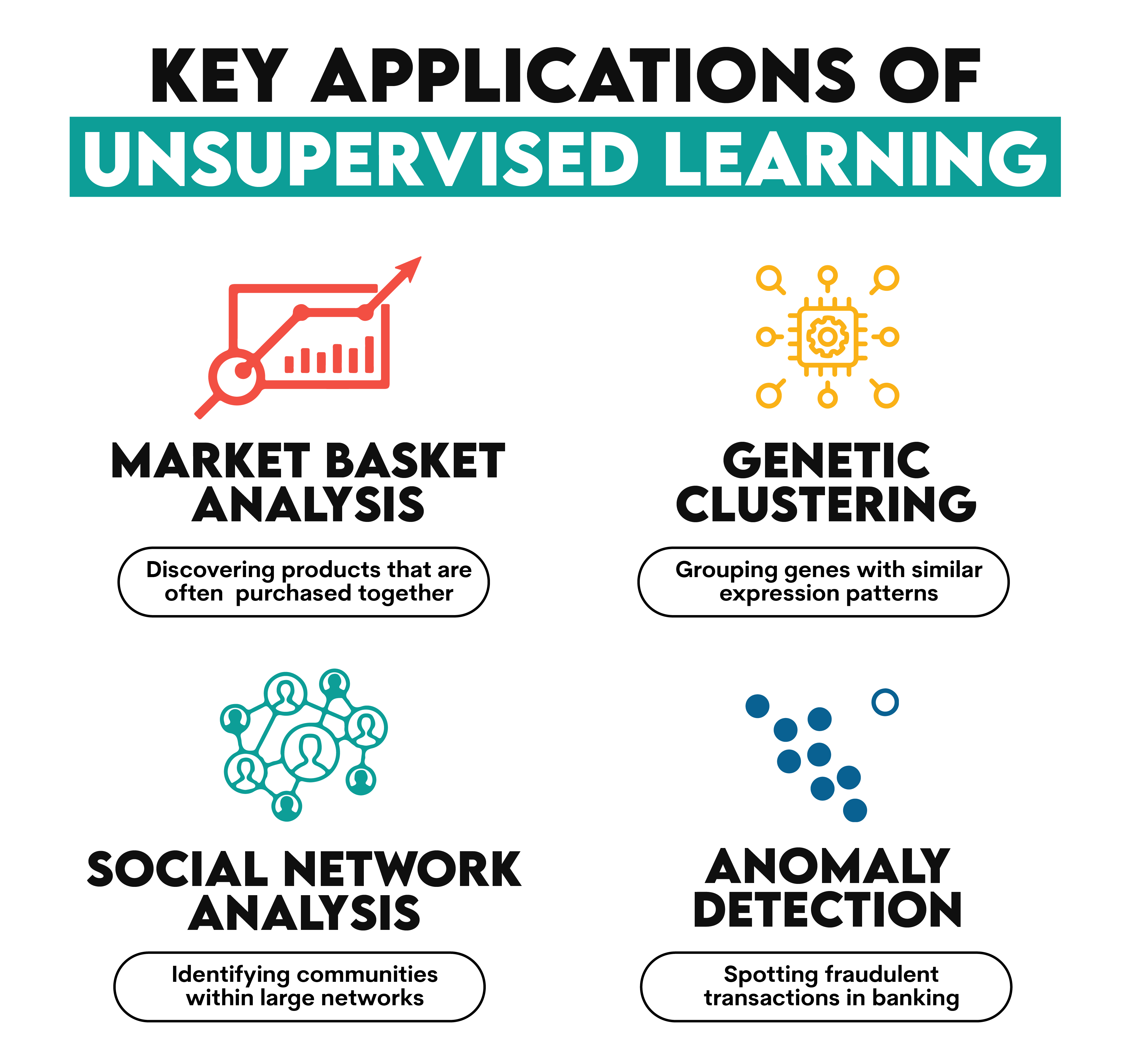
• Market basket analysis: Discovering products that are often purchased together.
• Genetic clustering: Grouping genes with similar expression patterns.
• Social network analysis: Identifying communities within large networks.
• Anomaly detection: Spotting fraudulent transactions in banking.

Advantages

Unsupervised Learning can uncover hidden patterns in data without labels, making it useful for exploratory data analysis. It's particularly valuable when unsure what you want in the data.

Limitations

However, the lack of labeled data makes validating the model's performance challenging. Additionally, interpreting the results of unsupervised learning algorithms can be more complex and subjective than supervised learning.

Popular algorithms

• K-means Clustering: Groups data into k number of clusters based on feature similarity.
• Hierarchical Clustering: Builds a tree of clusters by continually merging or splitting existing clusters.
• Principal Component Analysis (PCA): Reduces the dimensionality of data while retaining most of the variation.
• Autoencoders: Neural networks designed to compress data into a lower-dimensional representation and then reconstruct it.

Application of Unsupervised Learning

Now, let’s see the code. Again we first load the libraries.

from sklearn.cluster import KMeans, AgglomerativeClustering
from sklearn.metrics import silhouette_score
from sklearn.decomposition import PCA
from sklearn.neural_network import MLPRegressor

Next, let’s standardize the data, apply those algorithms, and add the results to the dictionary. We will compare them at the end.

# Standardize the data for clustering and autoencoder
scaler = StandardScaler()
X_scaled = scaler.fit_transform(X_wine)

# Apply K-means Clustering
kmeans = KMeans(n_clusters=3, random_state=42)  # We choose 3 as a starting point, as there are 3 classes of wine
kmeans.fit(X_scaled)
kmeans_labels = kmeans.labels_
kmeans_silhouette = silhouette_score(X_scaled, kmeans_labels)

# Apply Hierarchical Clustering
hierarchical = AgglomerativeClustering(n_clusters=3)  # Same number of clusters for comparison
hierarchical.fit(X_scaled)
hierarchical_labels = hierarchical.labels_
hierarchical_silhouette = silhouette_score(X_scaled, hierarchical_labels)

# Apply PCA
pca = PCA(n_components=0.95)  # Retain 95% of the variance
X_pca = pca.fit_transform(X_scaled)
pca_explained_variance = pca.explained_variance_ratio_.sum()

# Train an Autoencoder - For simplicity, we'll design a small one
autoencoder = MLPRegressor(hidden_layer_sizes=(32, 16, 32),
                           max_iter=2000,
                           random_state=42)
autoencoder.fit(X_scaled, X_scaled)
X_reconstructed = autoencoder.predict(X_scaled)
autoencoder_reconstruction_error = ((X_scaled - X_reconstructed) ** 2).mean()

# Compile the results
unsupervised_results = {
    'K-means Clustering': kmeans_silhouette,
    'Hierarchical Clustering': hierarchical_silhouette,
    'PCA Explained Variance': pca_explained_variance,
    'Autoencoder Reconstruction Error': autoencoder_reconstruction_error
}

unsupervised_results

Here is the output.

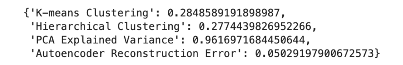
• K-means Clustering: A silhouette score of approximately 0.285 was achieved, which is a moderate score indicating that the clusters have some overlap.
• Hierarchical Clustering: Obtained a slightly lower silhouette score of about 0.277, suggesting a similar level of cluster overlap as K-means.
• PCA Explained Variance: The PCA retained about 96.17% of the dataset's variance, indicating a substantial reduction in dimensionality while preserving most of the information.
• Autoencoder Reconstruction Error: A low reconstruction error of approximately 0.050 means the autoencoder could compress and reconstruct the dataset with a small amount of error.

Reinforcement Learning

Reinforcement Learning (RL) is a type of machine learning where an agent learns to make decisions by taking actions in an environment to achieve some goals.

It's similar to training a pet with rewards and penalties: the agent learns the best actions to maximize rewards over time.

In RL, the agent interacts with its environment, receives feedback through rewards or penalties, and adjusts its strategy to improve future rewards. The learning process involves exploration (trying new things) and exploitation (using known information to gain rewards).

Key applications and examples

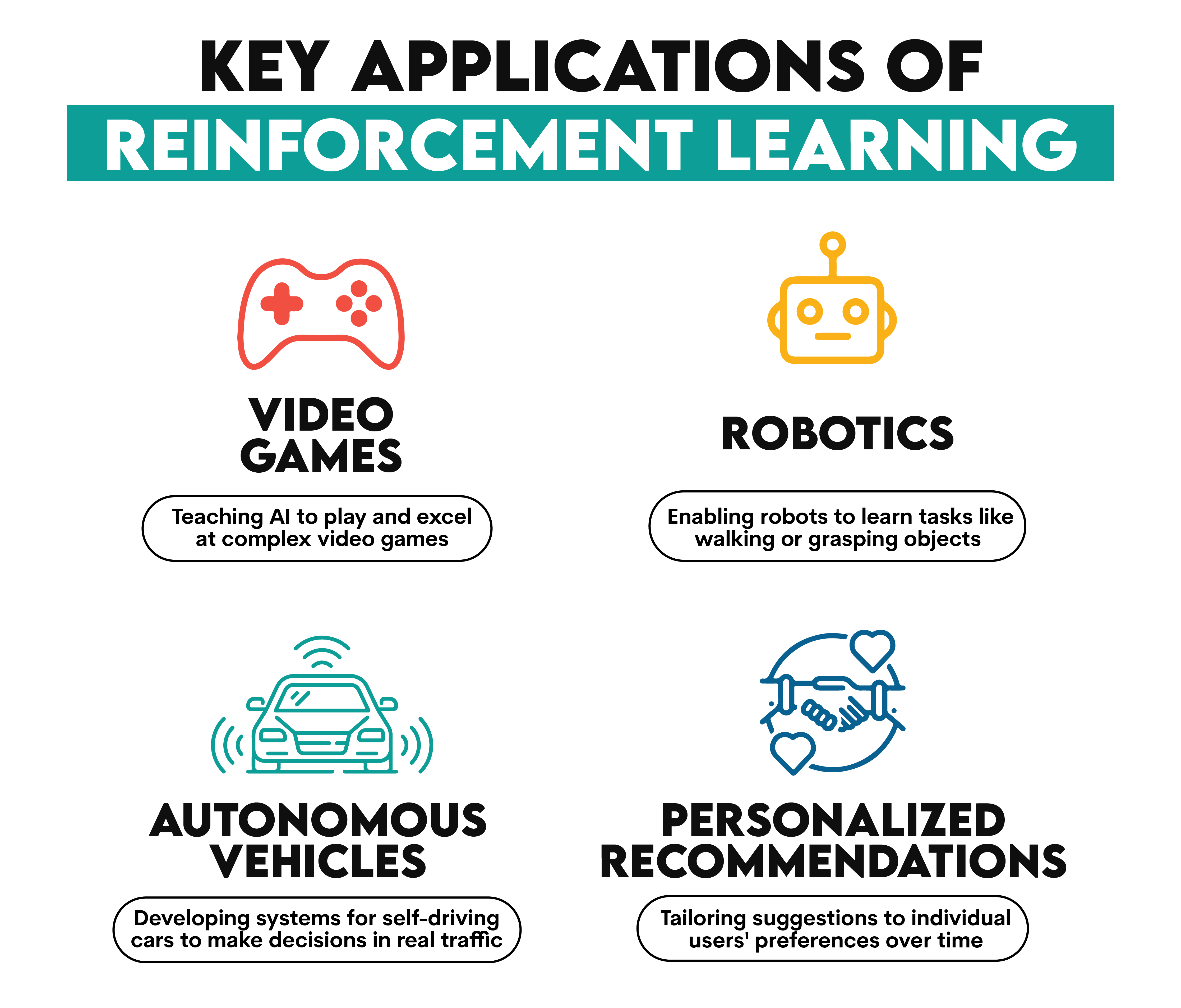
• Video games: Teaching AI to play and excel at complex video games.
• Robotics: Enabling robots to learn tasks like walking or grasping objects.
• Autonomous vehicles: Developing systems for self-driving cars to make decisions in real traffic.
• Personalized recommendations: Tailoring suggestions to individual users' preferences over time.

Advantages

Reinforcement Learning is powerful for tasks that involve making a series of judgements. It allows models to learn from the results of actions, which is helpful for complicated problems where it is difficult to express precise instructions.

Limitations

However, RL needs a large amount of data and processing power to learn successfully. It might be difficult to create the ideal system of rewards for direct learning without having unexpected results.

Popular algorithms

• Q-learning: A value-based method for learning the quality of actions, indicating the potential for reward.
• Deep Q Network (DQN): Combines Q-learning with deep neural networks to handle high-dimensional sensory input.
• Policy Gradient methods: Learn a policy directly that maps states to the probability of taking an action.

Other Types of Machine Learning

• Semi-supervised Learning is a hybrid approach that uses labeled and unlabeled data for training. It's useful when acquiring a fully labeled dataset is expensive or impractical. This method can improve learning accuracy with less labeled data.
• Self-supervised Learning is a form of unsupervised learning where the data provides supervision. The system learns to predict part of the input from other parts of the input using pretext tasks. It's particularly effective in scenarios where labeled data is scarce but unlabeled data is abundant.
• Federated Learning is a machine learning approach that trains an algorithm across multiple decentralized devices or servers holding local data samples, without exchanging them. This method is beneficial for privacy preservation and data security and reduces the need to centralize large datasets.

These approaches extend the capabilities of machine learning models by leveraging different data configurations and privacy considerations, opening up new possibilities for applications and efficiency improvements.

How to select the appropriate type of ML for different tasks and Projects?

Selecting the right machine learning type depends on several factors, including the nature of your data, the task at hand, and the resources available. Here are some considerations:

• Data availability and labeling: Supervised learning is often the best choice if you have a large labeled dataset. For unlabeled data, consider unsupervised learning. Semi-supervised or self-supervised learning can be powerful when you have limited labeled data.
• Task complexity and requirements: Reinforcement learning suits tasks requiring decision-making over time, like robotics or game playing. For classification or regression tasks, supervised learning algorithms are more appropriate.
• Privacy concerns: If data privacy is a concern, federated learning allows for training on decentralized data, preserving users' privacy.
• Computational resources: Reinforcement learning and deep learning models may require significant computational resources. Ensure your choice aligns with the available computational budget.
• Domain-specific considerations: Some fields, like bioinformatics or finance, may have specific requirements or prevalent practices that favor certain types of machine learning.
  

Understanding your project's specific needs and constraints is key to selecting the most appropriate machine-learning approach. This decision will impact your solution's effectiveness, efficiency, and scalability.

Final Thoughts

So, we've taken quite the tour through machine learning, dipping our toes in everything from the clear waters of different types of machine learning.

The key to being able to code these machine learning algorithms is not just in understanding them but also in rolling up your sleeves and getting your hands dirty with real-world projects, like the Doordash project, where the aim is to predict delivery duration.