Unsupervised Clustering: Methods, Examples, and When to Use

A practical guide to Unsupervised Clustering techniques, their use cases, and how to evaluate clustering performance.

We all know supervised clustering, where you have labeled data that guides you to categorize the input, but what if you don’t have labels, no guidance, no hint, just raw, unlabeled data?
That’s what most real-life data looks like; unsupervised clustering steps are needed in these situations. In this technique, we will group similar data points based solely on structure and distribution without an external input.

In this article, we will discover unsupervised clustering techniques and how to evaluate the results. We will also see real-world examples, how to choose the best clustering techniques, and common pitfalls to avoid while selecting unsupervised clustering techniques. Let’s start with the fundamentals.

What is Unsupervised clustering?

In supervised learning, there are labels. What are labels? Labels mean the feature you want to predict. For instance, you want to predict house prices.

• Supervised Learning
  • Scenario A: The Dataset has house prices.
• Unsupervised Learning
  • Scenario B: The dataset doesn’t have house prices.

So in unsupervised clustering, the dataset doesn’t have the label you want to predict, but you have to split it into clusters by following different logics, which we will see for each technique.

If you’re still unclear about how labeled and unlabeled data differ, check out this quick comparison on supervised vs unsupervised learning.

For a deeper breakdown of how unsupervised learning works overall (not just clustering), this guide on what is unsupervised learning is worth bookmarking.

Common Techniques in Unsupervised Clustering

Clustering algorithms help similar points find each other within data points. Each method we will discover will do the same thing with different methods, uncovering hidden groups.

K-Means Clustering

K-Means tries to find the center for each cluster at first. Then it assigns these centers as clusters, and here the “K” represents the number of clusters you want to define.

Unlike hierarchical clustering or DBScan, K-means assumes that clusters are spherical and their sizes are even.

In the code below, we will create synthetic data and four clusters.

from sklearn.datasets import make_blobs
from sklearn.cluster import KMeans
import matplotlib.pyplot as plt

# Generate synthetic data
X, _ = make_blobs(n_samples=2100, centers=4, cluster_std=0.7, random_state=0)

# Apply K-Means
kmeans = KMeans(n_clusters=4, random_state=0)
kmeans.fit(X)
y_kmeans = kmeans.predict(X)

# Visualize results
plt.scatter(X[:, 0], X[:, 1], c=y_kmeans, s=40, cmap='viridis')
plt.scatter(kmeans.cluster_centers_[:, 0], kmeans.cluster_centers_[:, 1], s=200, alpha=0.75, marker='X')
plt.title("K-Means Clustering")
plt.show()

Here is the output.

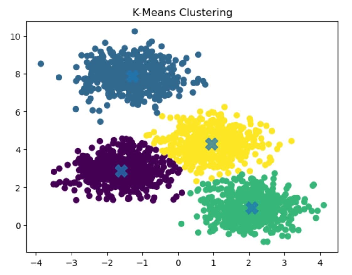
In this graph above, you see different centers and different clusters.

Hierarchical Clustering

Hierarchical Clustering creates groups step by step, like a tree's branches, and it does not need a fixed number of groups, unlike some other clustering methods.. We will make and group a dataset in the code below using hierarchical clustering.

from sklearn.datasets import make_blobs
from scipy.cluster.hierarchy import dendrogram, linkage
import matplotlib.pyplot as plt

X, _ = make_blobs(n_samples=30, cluster_std=0.7, random_state=0)

linked = linkage(X, method='ward')

plt.figure(figsize=(8, 4))
dendrogram(linked)
plt.title("Hierarchical Clustering - Dendrogram")
plt.xlabel("Sample index")
plt.ylabel("Distance")
plt.show()

Here is the output.

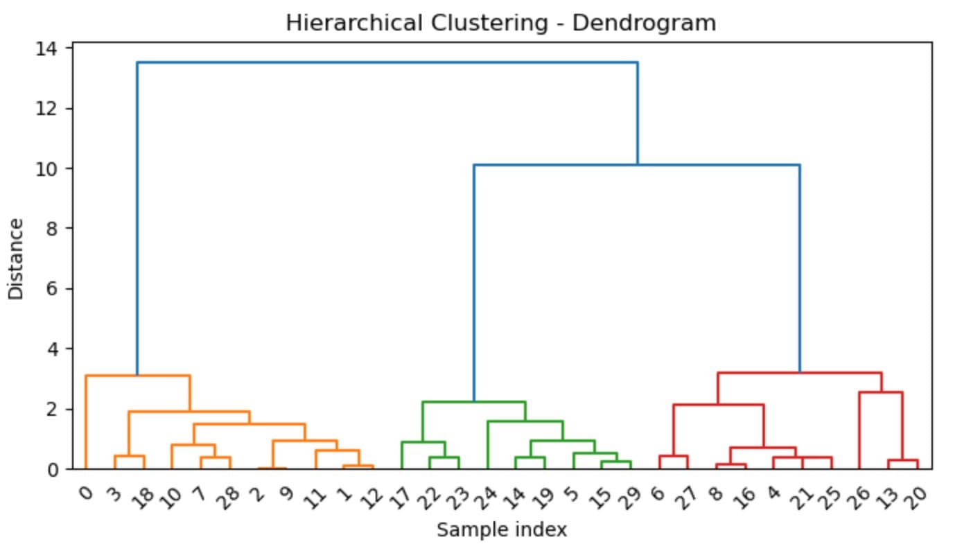
The output of the hierarchical clustering is also known as a dendrogram. In this dendrogram, you can see different branches, and at the end, there are 3 of them(check colors).

DBSCAN

DBScan groups data points based on the density. It is good when cluster shapes are irregular.

In the code below, we will generate data by changing densities and use DBSCAN to detect both compact clusters and outlier points.

from sklearn.datasets import make_blobs
from sklearn.cluster import KMeans
import matplotlib.pyplot as plt

X, _ = make_blobs(n_samples=300, centers=4, cluster_std=0.6, random_state=0)

kmeans = KMeans(n_clusters=4, random_state=0)
kmeans.fit(X)
y_kmeans = kmeans.predict(X)

plt.scatter(X[:, 0], X[:, 1], c=y_kmeans, s=40, cmap='viridis')
plt.scatter(kmeans.cluster_centers_[:, 0], kmeans.cluster_centers_[:, 1], s=200, alpha=0.75, marker='X')
plt.title("K-Means Clustering")
plt.show()

Here is the output.

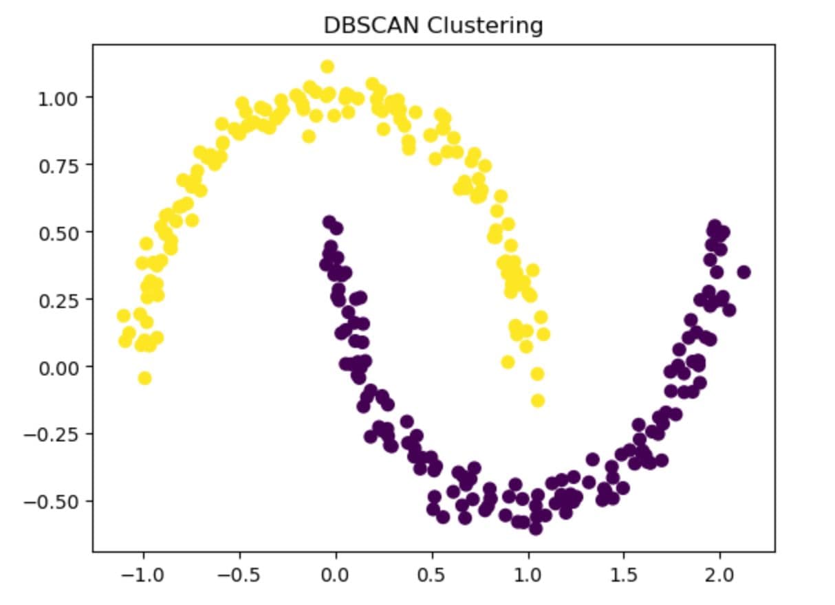
As you can see, DBSCAN finds two crescent-shaped clusters without knowing the number of groups.

Gaussian Mixture Models(GMM)

Gaussian Mixture Models assume that your data will be in a Gaussian distribution. It assigns probabilities to each point. This is called soft clustering, and you can see some data points overlap in the output.

Here is the code where you create data points first and apply GMM.

from sklearn.datasets import make_blobs
from sklearn.mixture import GaussianMixture
import matplotlib.pyplot as plt

X, _ = make_blobs(n_samples=300, centers=3, cluster_std=0.8, random_state=0)

gmm = GaussianMixture(n_components=3, random_state=0)
labels = gmm.fit_predict(X)

plt.scatter(X[:, 0], X[:, 1], c=labels, s=40, cmap='viridis')
plt.title("Gaussian Mixture Model Clustering")
plt.show()

Here is the output.

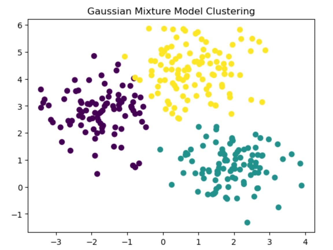
As you can see, three different soft clusters are shaped more like ellipses than circles. As you can see, GMM also allows overlap between groups to capture more subtle structure than K-Means.

Spectral Clustering

Special Clustering uses graph theory to split data based on connectivity, not just distance. That is why it is helpful to detect complex structures.

In this code, we will create a noisy circular dataset and apply spectral clustering.

from sklearn.datasets import make_circles
from sklearn.cluster import SpectralClustering
import matplotlib.pyplot as plt

X, _ = make_circles(n_samples=300, factor=0.5, noise=0.05)

spectral = SpectralClustering(n_clusters=2, affinity='nearest_neighbors', assign_labels='kmeans', random_state=0)
labels = spectral.fit_predict(X)

plt.scatter(X[:, 0], X[:, 1], c=labels, cmap='viridis', s=40)
plt.title("Spectral Clustering")
plt.show()

Here is the output.

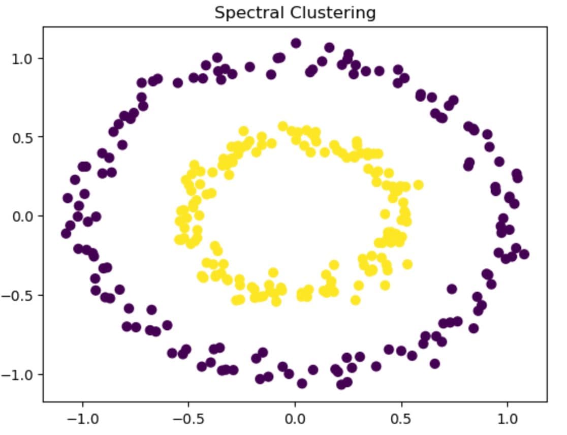
In this graph above, there are two clusters, one circle inside another. Typically, K-Means would fail, which is not good at separating the nested circles.

Choosing the Right Unsupervised Clustering Technique

Before performing the proper clustering method, you might feel confused. To decrease the number of our options, let’s see when each technique is best for and when to avoid using them.

K-Means Clustering

• Best for: Simple, round clusters that don’t overlap and are about the same size.
• Avoid if: Your data has outliers, noise, or strange shapes.

Hierarchical Clustering

• Best for: Small datasets where you want to see how groups build step by step.
• Avoid if: The data is extensive, because it can be slow and hard to process.

DBSCAN

• Best for: Clusters of any shape, especially if your data has noise or gaps.
• Avoid if: Your clusters are too close together, or setting the correct settings is hard.

Gaussian Mixture Models (GMM)

• Best for: Groups that may overlap and aren’t perfect circles.
• Avoid if: You want clear, separate groups with no mixing.

Spectral Clustering

• Best for: Complex patterns or when groups connect in tricky ways.
• Avoid if: You have a lot of data, it takes more time and memory.

Evaluation of Unsupervised Clustering Results

Unlike supervised learning, clustering does not give you a score at once. There are not only labels, so we need to use different metrics to evaluate how good our groupings are.

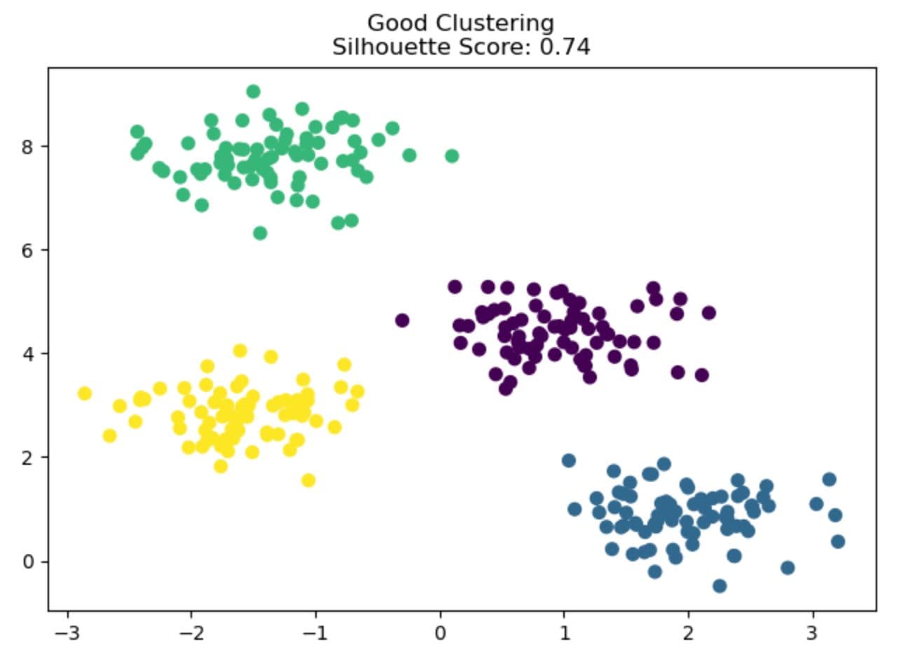
1. Silhouette Score

This index shows how well a point fits in its cluster vs. others. Values range from -1 to 1; closer to 1 means better separation.

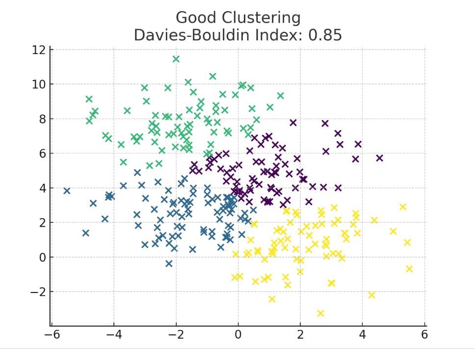
2. Davies-Boulding Index

This measures how close and far apart these clusters are, with a lower mean, tighter, and better-separated groups.

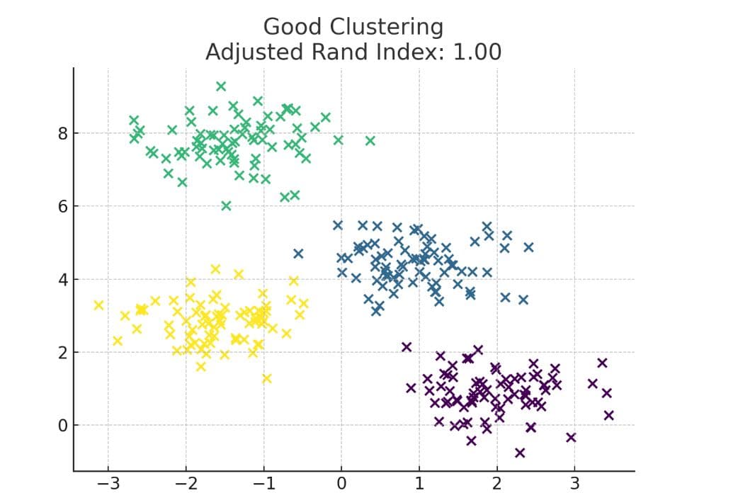
3. Adjusted Rand Index

This compares your clustering to real labels. A score near one means they match closely.

Real-World Applications of Unsupervised Clustering

Now, these examples might be a little abstract for you, so let’s give some real-world examples.

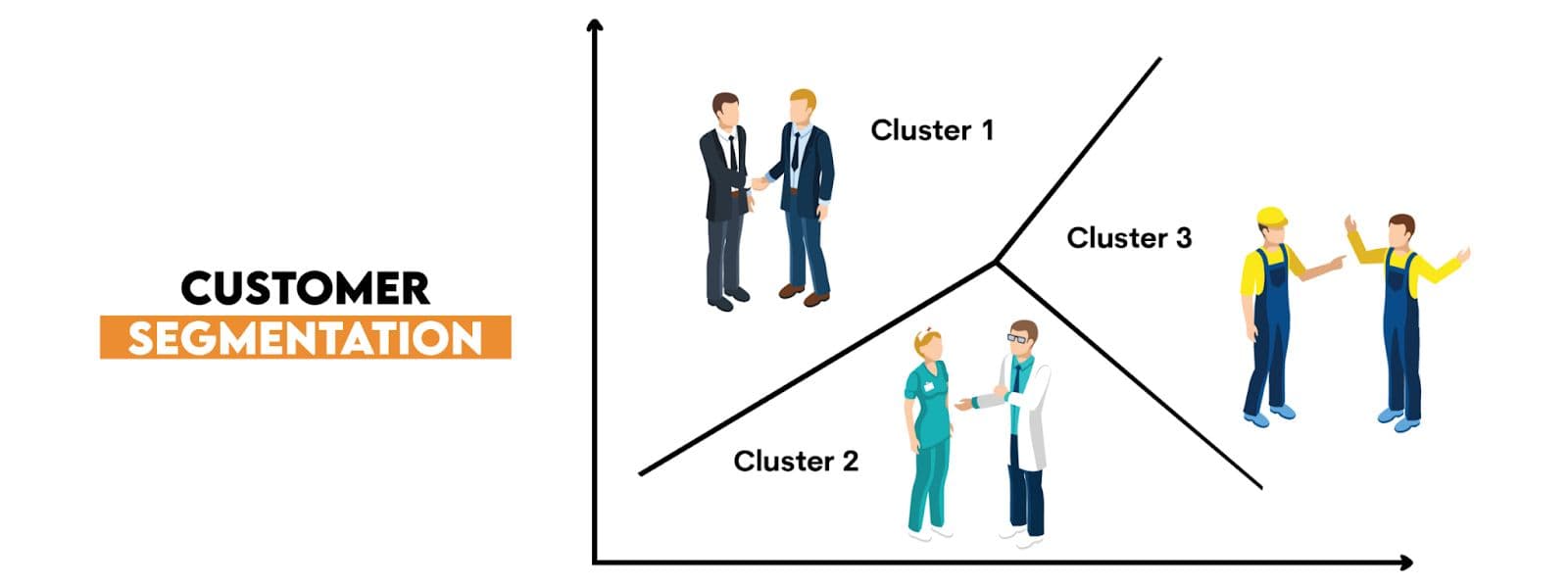
Customer Segmentation

Putting customers into different clusters would help retailers to discover their buying patterns, which helps reduce the marketing cost of these companies.

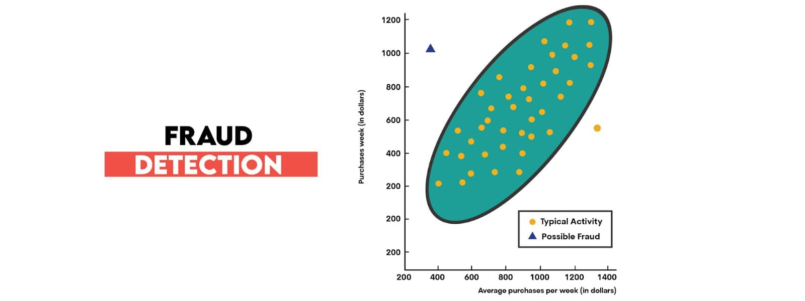
Anomaly Detection

In finance, DBSCAN spots outliers and detects irregular data points. It is good to do fraud detection, for instance.

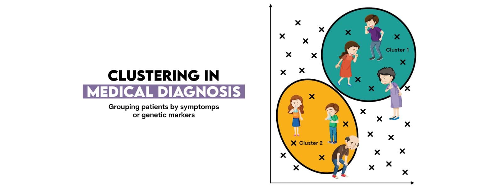
Medical Diagnosis

In medical diagnosis, clustering groups of patients by symptoms or genetic markers

Conclusion

Unsupervised clustering helps you find patterns in data without labels. Each method works best in different situations, so it's important to choose the one that fits your data. Use simple metrics to check if your clusters make sense. Always think about what the results mean in real life.