The Pandas Cheat Sheet To Be a Better Data Scientist


Here is Pandas cheat sheet explaining the functions any data scientist should know. Included are interview questions from Forbes, Meta, Google, and Amazon.
Characteristics of Pandas in Python
Pandas is an open-source Python library. It is used for data analysis and manipulation and was created by Wes Kinney in 2008.
It is also one of the most commonly used libraries in Machine Learning, making its community highly active and popular.
Oftentimes, you can see that Numpy also will be imported when importing Pandas. It’s because most NumPy functions also work on DataFrames, the typical Pandas data structure.
What Is Pandas Cheat Sheet and Why Do We Need One?
The cheat sheets are used by students in the exam without their teacher's knowledge to, well, cheat.
Yet, the term will differ in programming. In Python programming, cheat sheets include a summary of the codes with quick explanations and demonstrations. It will help you to memorize the codes and map them into your mind.
Also, it works when you need to remind yourself about some specific function.
Which function works best for finding missing values or exploring data? Which function to use to filter columns?
When you encounter that kind of problem, you can easily open the cheat sheet and recall it.
Pandas cheat sheet will help you look up the Pandas library features like operations in DataFrames, such as locating, filtering, or finding missing values, exploring data, reading data, or even making data visualization.
So let’s get into the Pandas Cheat Sheet by explaining Pandas basics first.
Pandas Cheat Sheet for Data Science
Pandas Basics
Now, let’s start this Pandas cheat sheet by explaining Panda’s Basics, like data structures. After that section, we will go deeper into functions with examples from the platform.
Now, before starting, let’s see How to Import Pandas as pd in Python.
Pandas Data Structures
We have two different data structures in Pandas, series, and DataFrames.
Series
The Pandas series is the first data structure of Pandas. It’s a type of data structure where we can assign different data types as an index, and it also can store different data types.
DataFrames
DataFrames are multi-dimensional, size-mutable data structures with columns and can store different types of data.
It can look like the multiplication of different series or SQL tables.
The image below shows how the data is organized in Series and DataFrames, respectively.

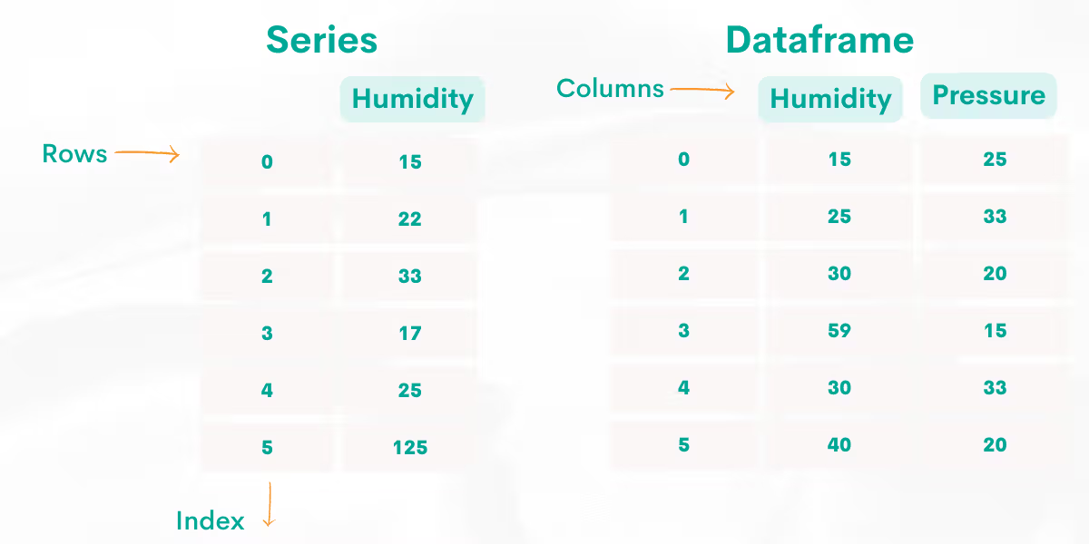
For a quick overview of these two data structures differ, take a look at the image below.

DataFrame Manipulation
Now, in this section of Pandas cheat sheet, we will explore the functions used for DataFrame manipulation in Pandas in the following sub-sections:
- Data Exploring
- Data Retrieving
- Data Operations
- Duplicate & Missing Values
- Merging
- Plotting
- Saving From and Reading To DataFrame
- DateTime
Data Exploring
Before starting analyzing your data, the following image will give you a great summary of the data exploring functions.
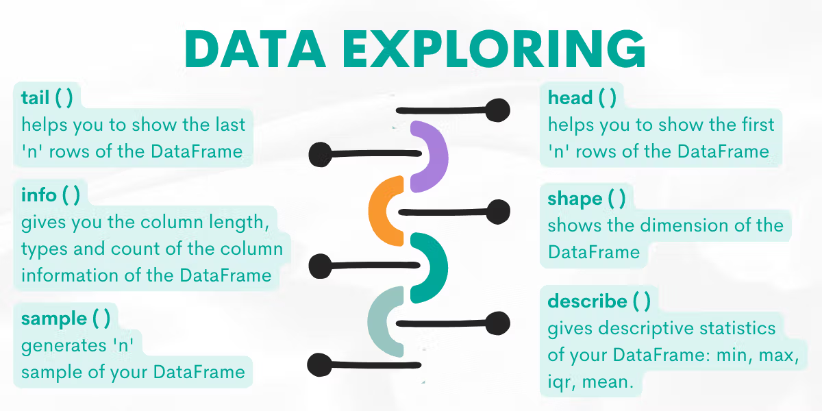
Let’s explore them by giving examples from the platform.
Function: head( )
This function will give you the “n” head rows of your DataFrame. If you run this function without an argument, it will output 5 rows.
Syntax
The function’s syntax is:
DataFrame.head(n=5)For a detailed explanation, please refer to the official Pandas documentation.
Example
Here is the question that we’ll use to show you how this function works.
Find the country that has the most companies listed on Forbes.
Output the country along with the number of companies.
The question asks us to find the country with the most companies listed on Forbes.
By running the head( ) function without an argument like below, it will return the first 5 rows.
forbes_global_2010_2014.head()| company | sector | industry | continent | country | marketvalue | sales | profits | assets | rank | forbeswebpage |
|---|---|---|---|---|---|---|---|---|---|---|
| ICBC | Financials | Major Banks | Asia | China | 215.6 | 148.7 | 42.7 | 3124.9 | 1 | http://www.forbes.com/companies/icbc/ |
| China Construction Bank | Financials | Regional Banks | Asia | China | 174.4 | 121.3 | 34.2 | 2449.5 | 2 | http://www.forbes.com/companies/china-construction-bank/ |
| Agricultural Bank of China | Financials | Regional Banks | Asia | China | 141.1 | 136.4 | 27 | 2405.4 | 3 | http://www.forbes.com/companies/agricultural-bank-of-china/ |
| JPMorgan Chase | Financials | Major Banks | North America | United States | 229.7 | 105.7 | 17.3 | 2435.3 | 4 | http://www.forbes.com/companies/jpmorgan-chase/ |
| Berkshire Hathaway | Financials | Investment Services | North America | United States | 309.1 | 178.8 | 19.5 | 493.4 | 5 | http://www.forbes.com/companies/berkshire-hathaway/ |
Also, we can use it with arguments like that.
forbes_global_2010_2014.head(7)
Here is the output.
| company | sector | industry | continent | country | marketvalue | sales | profits | assets | rank | forbeswebpage |
|---|---|---|---|---|---|---|---|---|---|---|
| ICBC | Financials | Major Banks | Asia | China | 215.6 | 148.7 | 42.7 | 3124.9 | 1 | http://www.forbes.com/companies/icbc/ |
| China Construction Bank | Financials | Regional Banks | Asia | China | 174.4 | 121.3 | 34.2 | 2449.5 | 2 | http://www.forbes.com/companies/china-construction-bank/ |
| Agricultural Bank of China | Financials | Regional Banks | Asia | China | 141.1 | 136.4 | 27 | 2405.4 | 3 | http://www.forbes.com/companies/agricultural-bank-of-china/ |
| JPMorgan Chase | Financials | Major Banks | North America | United States | 229.7 | 105.7 | 17.3 | 2435.3 | 4 | http://www.forbes.com/companies/jpmorgan-chase/ |
| Berkshire Hathaway | Financials | Investment Services | North America | United States | 309.1 | 178.8 | 19.5 | 493.4 | 5 | http://www.forbes.com/companies/berkshire-hathaway/ |
| Exxon Mobil | Energy | Oil & Gas Operations | North America | United States | 422.3 | 394 | 32.6 | 346.8 | 6 | http://www.forbes.com/companies/exxon-mobil/ |
| General Electric | Industrials | Conglomerates | North America | United States | 259.6 | 143.3 | 14.8 | 656.6 | 7 | http://www.forbes.com/companies/general-electric/ |
This time we showed 7 first rows. So when the function takes “n” as an argument, it will return the DataFrame's first “n” rows.
You can also continue solving this question, yet this will be enough for talking about the head( ) function.
Function: sample( )
The sample function returns “n” rows of the DataFrame, which are randomly selected.
Syntax
The function’s syntax is:
DataFrame.sample(n=None, frac=None, replace=False, weights=None, random_state=None, axis=None, ignore_index=False)For a detailed explanation, please refer to the official Pandas documentation.
Example
Now, if you look closer, our DataFrame contains a rank column and is sorted. When exploring DataFrames, it is good to see the information randomly.
We will use the same question for this function.
To see three random rows from the DataFrame, we will use 3 as an argument in the sample( ) function.
Let’s see the code.
import pandas as pd
forbes_global_2010_2014.sample(3)
Here is the output.
| company | sector | industry | continent | country | marketvalue | sales | profits | assets | rank | forbeswebpage |
|---|---|---|---|---|---|---|---|---|---|---|
| Royal Bank of Canada | Financials | Major Banks | North America | Canada | 95.7 | 37.8 | 8 | 811.4 | 55 | http://www.forbes.com/companies/royal-bank-of-canada/ |
| Ford Motor | Consumer Discretionary | Auto & Truck Manufacturers | North America | United States | 64.5 | 146.9 | 7.2 | 202 | 47 | http://www.forbes.com/companies/ford-motor/ |
| Cisco Systems | Information Technology | Communications Equipment | North America | United States | 119 | 47.9 | 8.2 | 98.4 | 82 | http://www.forbes.com/companies/cisco-systems/ |
Now, do not forget once you call this function on your own, it will return different rows.
Function: describe( )
It will return descriptive statistics of your DataFrames, which are count, mean, %25, %50 % 75 (lower and upper percentiles), and a max of the columns.
Syntax
The function’s syntax is:
DataFrame.describe(percentiles=None, include=None, exclude=None, datetime_is_numeric=False)For a detailed explanation, please refer to the official Pandas documentation.
Example
Now, if we will work with numbers, this function is very useful. We will use the same question as above.
To understand better how our function will work, let’s see the DataFrame columns first.
| company | sector | industry | continent | country | marketvalue | sales | profits | assets | rank | forbeswebpage |
|---|---|---|---|---|---|---|---|---|---|---|
| ICBC | Financials | Major Banks | Asia | China | 215.6 | 148.7 | 42.7 | 3124.9 | 1 | http://www.forbes.com/companies/icbc/ |
| China Construction Bank | Financials | Regional Banks | Asia | China | 174.4 | 121.3 | 34.2 | 2449.5 | 2 | http://www.forbes.com/companies/china-construction-bank/ |
| Agricultural Bank of China | Financials | Regional Banks | Asia | China | 141.1 | 136.4 | 27 | 2405.4 | 3 | http://www.forbes.com/companies/agricultural-bank-of-china/ |
| JPMorgan Chase | Financials | Major Banks | North America | United States | 229.7 | 105.7 | 17.3 | 2435.3 | 4 | http://www.forbes.com/companies/jpmorgan-chase/ |
| Berkshire Hathaway | Financials | Investment Services | North America | United States | 309.1 | 178.8 | 19.5 | 493.4 | 5 | http://www.forbes.com/companies/berkshire-hathaway/ |
Let’s see the code.
import pandas as pd
forbes_global_2010_2014.describe()
Here is the output.
| marketvalue | sales | profits | assets | rank |
|---|---|---|---|---|
| 100 | 100 | 100 | 100 | 100 |
| 136.536 | 112.39 | 11.836 | 595.083 | 50.44 |
| 85.78 | 91.541 | 8.514 | 730.084 | 28.94 |
| 38.9 | 27.7 | 3.3 | 69.9 | 1 |
| 75.25 | 54.875 | 6 | 141.3 | 25.75 |
| 102.6 | 87.3 | 8.8 | 246.45 | 50.5 |
| 184.7 | 129.45 | 14.8 | 700.45 | 75.25 |
| 483.1 | 476.5 | 42.7 | 3124.9 | 100 |
It only outputs the integer and float values.
Function: tail( )
This function will return the last “n” row of the data set. If you use this function without an argument, it will automatically return the last 5 rows.
Syntax
The function’s syntax is:
DataFrame.tail(n=5)[source]For a detailed explanation, please refer to the official Pandas documentation.
Example
The question asks us to find the last five records of the dataset.
Find the last five records of the dataset.
Here, we will use the tail function with 5 as an argument.
Let’s see the code.
import pandas as pd
import numpy as np

result = worker.tail(5)
Here is the output.
| worker_id | first_name | last_name | salary | joining_date | department |
|---|---|---|---|---|---|
| 8 | Geetika | Chauhan | 90000 | 2014-04-11 00:00:00 | Admin |
| 9 | Agepi | Argon | 90000 | 2015-04-10 00:00:00 | Admin |
| 10 | Moe | Acharya | 65000 | 2015-04-11 00:00:00 | HR |
| 11 | Nayah | Laghari | 75000 | 2014-03-20 00:00:00 | Account |
| 12 | Jai | Patel | 85000 | 2014-03-21 00:00:00 | HR |
Function: shape( )
This function will give you the dimensions of the DataFrame. Simply said, it returns the number of rows and columns.
Syntax
The function’s syntax is:
DataFrame.shapeFor a detailed explanation, please refer to the official Pandas documentation.
Example
Here is the question.
Interview Question Date: June 2018
Find the ratio of successfully received messages to sent messages.
This question asks us to find the ratio of successfully received and sent messages. We have two DataFrames, and to find the ratio, we will divide receiving messages into sent messages.
To find the length of the first DataFrame, we will use the shape function with zero.
Why?
Because the shape function returns a tuple. It shows the dimension of the DataFrame, which is the length of the rows and columns, respectively. So when we select the first element of this output, we find the number of the rows of the DataFrame.
For this problem, we need the length of the rows so that we will select the first element of our output. To do that, we will use an index bracket with zero. If we want to find the length of the columns, we will use an index bracket with one.
Let’s see the code.
# Import your libraries
import pandas as pd
facebook_messages_received.shape[0]
Here is the first element of this tuple, which is the number of rows of the DataFrame.(length)
So to find the ratio, we will divide both DataFrames lengths (row number) each other.
Let’s see the code.
# Import your libraries
import pandas as pd

# Start writing code
result =  facebook_messages_received.shape[0] / facebook_messages_sent.shape[0]
Here is the output.
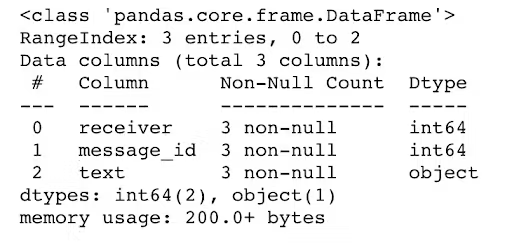
Function: info( )
This function will give you the columns' length information, with column types and the column count.
Syntax
The function’s syntax is:
DataFrame.info(verbose=None, buf=None, max_cols=None, memory_usage=None, show_counts=None, null_counts=None)For a detailed explanation, please refer to the official Pandas documentation.
Example
We can use this method on our previous question. In the code below, we will use this function without argument.
Let’s see how it works.
# Import your libraries
import pandas as pd

# Start writing code

facebook_messages_received.info()
Here is the output.

Data Retrieving
When you retrieve the data you want and filter, group, or sort it, you will use the following functions. The next function in our Pandas cheat sheet is data retrieving. Below’s a handy overview of these functions.
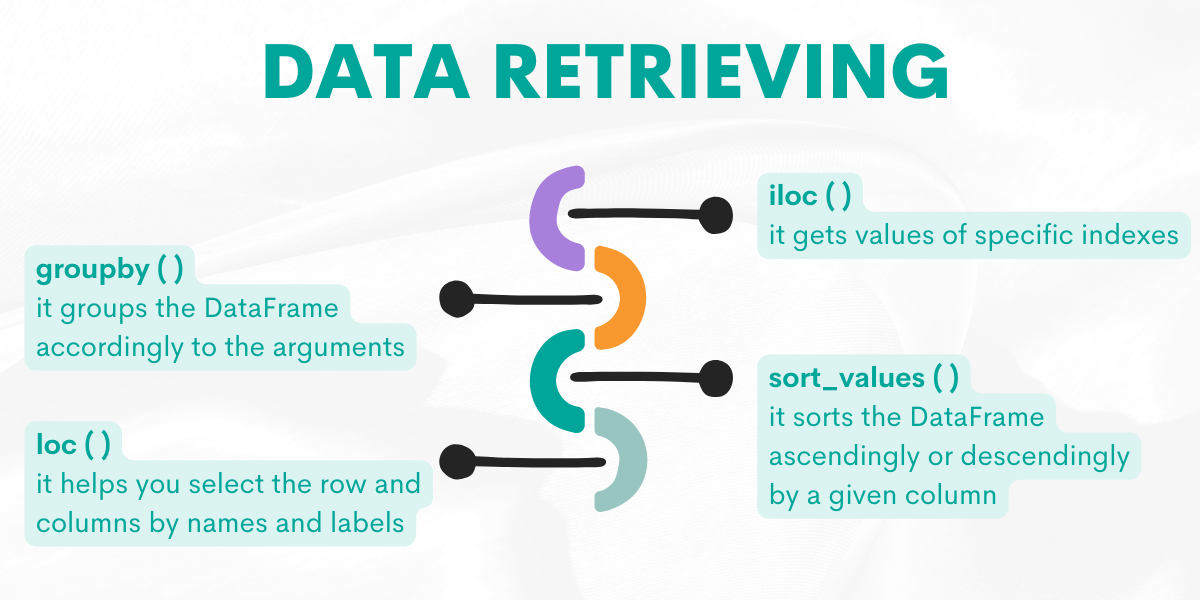
Let’s explore them by giving examples from the platform.
Function: iloc( )
This function will help you to get values of the specific indexes.
Syntax
The function’s syntax is:
DataFrame.ilocFor a detailed explanation, please refer to the official Pandas documentation.
Example
Here is the question.
Find employees who started in June and have even-numbered employee IDs.
This question asks us to return the workers who have an even-numbered worker id, by using colon indexing.
The logic behind the colon indexing is as follows;
X[start:stop:step]
When you don't define any of these “start-stop-step” arguments, they default to the values start = 0, stop = size of the dimension, step = 1.
Let’s see the code.
import pandas as pd

worker.iloc[1::2]
Here is the output.
| worker_id | first_name | last_name | salary | joining_date | department |
|---|---|---|---|---|---|
| 2 | Niharika | Verma | 80000 | 2014-06-11 00:00:00 | Admin |
| 4 | Amitah | Singh | 500000 | 2014-02-20 00:00:00 | Admin |
| 6 | Vipul | Diwan | 200000 | 2014-06-11 00:00:00 | Account |
| 8 | Geetika | Chauhan | 90000 | 2014-04-11 00:00:00 | Admin |
| 10 | Moe | Acharya | 65000 | 2015-04-11 00:00:00 | HR |
| 12 | Jai | Patel | 85000 | 2014-03-21 00:00:00 | HR |
So what if the question asks us to find the workers who have odd numbered worker_id?
Let’s see the code.
import pandas as pd
worker.head()

worker.iloc[::2]
Here is the output.
| worker_id | first_name | last_name | salary | joining_date | department |
|---|---|---|---|---|---|
| 1 | Monika | Arora | 100000 | 2014-02-20 00:00:00 | HR |
| 3 | Vishal | Singhal | 300000 | 2014-02-20 00:00:00 | HR |
| 5 | Vivek | Bhati | 500000 | 2014-06-11 00:00:00 | Admin |
| 7 | Satish | Kumar | 75000 | 2014-01-20 00:00:00 | Account |
| 9 | Agepi | Argon | 90000 | 2015-04-10 00:00:00 | Admin |
| 11 | Nayah | Laghari | 75000 | 2014-03-20 00:00:00 | Account |
Tip
X[start:stop: step]
Remember, Python is a zero-indexed coding language, which means the first index will be zero.
But if you assign one of your columns as an index, like worker_id in this question, and if your index starts at 1, then this code will return even elements.
(Here is the informative article about zero indexing.)
Yet, if you worked with a DataFrame, in which indexes start from zero, the following code returns odd elements.
import pandas as pd

df[1::2]
Function : groupby( )
It groups the DataFrame according to the arguments. It takes many arguments but probably the most used one is by. By equating this argument to the column name, you select how to group your DataFrame.
Syntax
The function’s syntax is:
DataFrame.groupby(by=None, axis=0, level=None, as_index=True, sort=True, group_keys=_NoDefault.no_default, squeeze=_NoDefault.no_default, observed=False, dropna=True)For a detailed explanation, please refer to the official Pandas documentation.
Example
Here is the question for practicing this function.
Interview Question Date: July 2020
Find the total AdWords earnings for each business type. Output the business types along with the total earnings.
This question asks us to find the total AdWords earnings for each business type. The question gave as a tip by saying “for each”. This phrase generally points you to use the groupby( ) function.
So let’s group by our DataFrame, and select business type because our question wants us to find AdWords earnings for each business type. To find the total, we will use the sum( ) function.
After that, we will use the reset index function to remove indexes that group by adds in the first place.
Let’s see the code.
import pandas as pd
import numpy as np

result = google_adwords_earnings.groupby(['business_type'])['adwords_earnings'].sum().reset_index()
Here is the output.
| business_type | adwords_earnings |
|---|---|
| handyman | 6042187 |
| media | 247914579 |
| transport | 132323280 |
Function: sort_values( )
It helps you sort the DataFrame according to the specified arguments.
This function can take many arguments, yet here are the two important ones.
The first one is by, which will define the value you want to sort. The second one is ascending; it defines how the DataFrame will be sorted. If you want to see values in descending order, meaning the highest value will be at the top, then you have to set ascending = False. Otherwise, ascending = True.
Syntax
The function’s syntax is:
DataFrame.sort_values(by, *, axis=0, ascending=True, inplace=False, kind='quicksort', na_position='last', ignore_index=False, key=None))For a detailed explanation, please refer to the official Pandas documentation.
Example
Here is the question.
Find quarterbacks that made most attempts to throw the ball in 2016. Output the quarterback along with the corresponding number of attempts. Sort records by the number of attempts in descending order.
The question asks us to find quarterbacks that made the most attempts to throw the ball in 2016. The question wants you to sort the values from the dataset in descending order.
First, we will select the year 2016. Then we will group the DataFrame by the name of quarterbacks, select the attempts, then assign the result to the DataFrame, and remove the indexes.
Now comes the sort_values( ) function, so let’s focus. Here we will sort values by times in descending order, meaning the highest number will be at the top.
Let’s see the code.
import pandas as pd
import numpy as np
y_2016 = qbstats_2015_2016[qbstats_2015_2016['year'] == 2016]
result = y_2016.groupby(['qb'])['att'].sum().to_frame('times').reset_index().sort_values('times', ascending = False)
Here is the output.
| qb | times |
|---|---|
| Drew BreesD. Brees | 673 |
| Joe FlaccoJ. Flacco | 672 |
| Aaron RodgersA. Rodgers | 610 |
| Carson PalmerC. Palmer | 597 |
| Philip RiversP. Rivers | 578 |
Function: loc( )
This function helps you to find the row and columns by labels, booleans, indexes, or callable functions.
You can pass this function with a list of labels [[“label1”, “label2” ]], or the conditions which will return booleans df.loc[df[“labels”'] > 6].
Syntax
The function’s syntax is:
DataFrame.locFor a detailed explanation, please refer to the official Pandas documentation.
Example
Here is the question.
Find the most expensive products on Amazon for each product category. Output category, product name and the price (as a number)
This question asks us to find the most expensive products on Amazon for each product category. The desired output contains the category, product name, and price.
First, we remove the dollar sign by using the replace( ) method. After that, we will change its type because we will use the idxmax function in the next step.
Next, we will group our DataFrame on product category, find the most expensive product using idxmax( ), then select category, product name, and price by bracket indexing.
Let’s focus on what the loc function does here. We will use the loc( ) function with two labels.
The first label helps us find the most expensive products on Amazon for each product category by using the group by function with the idxmax function.
The second label outputs the category, product name, and price.
Let's see the code.
import pandas as pd
import numpy as np
innerwear_amazon_com['price'] = innerwear_amazon_com['price'].replace(
    '[\$,]', '', regex=True).astype(float)
innerwear_amazon_com.loc[innerwear_amazon_com.groupby(['product_category'])['price'].idxmax(), ['product_category', 'product_name', 'price']]
Here is the output.
| product_category | product_name | price |
|---|---|---|
| Bras | Wacoal Women's Retro Chic Underwire Bra | 69.99 |
| Panties | Calvin Klein Women's Ombre 5 Pack Thong | 59.99 |
Data Operations
If you want to change the DataFrame according to your project needs or calculate the desired output, these data operations functions will help you do that. So, the next function in our Pandas cheat sheet is data operations.
For a quick reference, here’s the functions overview.


Now, let’s explain them by giving examples from the platform.
Function: agg( )
This function will pass one or multiple functions to columns/rows and rename the index of the resulting DataFrame, which can produce aggregated results.
Syntax
The function’s syntax is:
DataFrame.agg(func=None, axis=0, *args, **kwargs)It can work with a list of functions [np, sum, “max” ], function name as a string (‘min’) or dict like {'A' : ['sum', 'min'], 'B' : ['min', 'max']}
For a detailed explanation, please refer to the official Pandas documentation.
Example
Here is the question.
Interview Question Date: February 2021
How many customers placed an order and what is the average order amount?
This question asks us to find the number of customers with an order and the average order amount.
To do that, we will use the agg( ) function.
First, we will pass the nunique function to the customer_id column to find unique customers.
Second, we will use the mean function in the amount column to find an average order amount.
Agg( ) function can pass different functions for the different columns.
Here is the code.
import pandas as pd

result = postmates_orders.agg({'customer_id':'nunique', 'amount':'mean' }).reset_index()
Here is the output.
| index | 0 |
|---|---|
| customer_id | 5 |
| amount | 139.225 |
Function: apply( )
The apply( ) function allows you to perform operations on columns, rows, or entire DataFrames. It is only allowed to work with functions. It can produce aggregated results and works with multiple series at a time.
Syntax
The function’s syntax is:
DataFrame.apply(func, axis=0, raw=False, result_type=None, args=(), **kwargs)
For a detailed explanation, please refer to the official Pandas documentation.
Example
We will practice this function on this question.
Find the date when Apple's opening stock price reached its maximum
Forbes asks us to find the date when Apple’s opening stock price reached its maximum.
In this question, we will use the apply( ) function to change the date column format by defining a custom function with lambda. This lambda function takes the date column first. Then changes it by using the strftime( ) function.
The argument of the strftime( ) function is Y-M-D, which means this function will change the date column to Year-Month-Day format.
Finally, we will use the max( ) function in the date column to find the maximum stock price of Apple.
Let’s see the code.
import pandas as pd
import numpy as np
import datetime, time

df = aapl_historical_stock_price
df['date'] = df['date'].apply(lambda x: x.strftime('%Y-%m-%d'))

result = df[df['open'] == df['open'].max()][['date']]
Here is the output.
| date |
|---|
| 2012-09-21 |
Function: transform( )
This function allows you to broadcast functions to change individual columns. It works with a function, a string function, and a list of functions.
The transform( ) function can work with single series at a time but can not produce aggregated results.
Syntax
The function’s syntax is:
DataFrame.transform(func, axis=0, *args, **kwargs)
For a detailed explanation, please refer to the official Pandas documentation.
Example
Here is the question.
Find companies that have at least 2 Chinese speaking users.
Google asks us to find companies that have at least 2 Chinese-speaking users.
To do that, we will find the users who speak Chinese first. The question wants us to find companies, so we will use the groupby( ) function after that to find the number of users.
We will also use the transform( ) function with the count argument. Then we will use bracket indexing with conditions to find companies with at least 2 users.
Let’s see the code.
import pandas as pd

df_chinese = playbook_users[playbook_users.language == 'chinese']
df_chinese['n_users'] = df_chinese.groupby(['company_id'])['user_id'].transform('count')
df_chinese[df_chinese['n_users']>=2]['company_id'].unique()
Here is the output.
| 0 |
|---|
| 4 |
Function: drop( )
This function helps us remove DataFrames columns, rows, or columns and rows.
Syntax
The function’s syntax is:
DataFrame.drop(labels=None, *, axis=0, index=None, columns=None, level=None, inplace=False, errors='raise')
For a detailed explanation, please refer to the official Pandas documentation.
Example
Here is the question.
You have been asked to calculate the total salary for each department. Provide the salary as well as the corresponding department.
In this question, Amazon asks us to find the total salary of each department. Let’s search the keywords in this question to decode it.
We see “each” and “total”, which indicates we should use the groupby( ) and sum( ) functions together. After using the groupby( ) function, we will generally use reset_index( ) to remove indexes that the groupby( ) function adds and add Python indexes starting from zero.
We also have to remove the worker_id column because the question wants us to return only the salary with the department. To remove worker_id, we will use the drop( ) method with column name and axis argument as one. When equaling the axis argument to one, that means we want to remove the column and rename the salary column to sum.
Let’s see the code.
import pandas as pd

result= worker.groupby(['department']).sum().reset_index().drop('worker_id',axis = 1).rename(columns={"salary": "sum"})
Here is the output.
| department | sum |
|---|---|
| Account | 350000 |
| Admin | 1260000 |
| HR | 550000 |
Function: drop_duplicates( )
This function helps us to remove duplicate values in rows. By equaling inplace = “True” or “False”, you have the option to change the DataFrame.
Syntax
The function’s syntax is:
DataFrame.drop_duplicates(subset=None, *, keep='first', inplace=False, ignore_index=False)For a detailed explanation, please refer to the official Pandas documentation.
Example
Here is the question.
Find unique names women who participated in an Olympics before World War 2. Let's consider the year 1939 as the start of WW2.
Here, we will find the names of women who participated in the Olympics before World War 2. (1939). First, we will select females using the condition that the year has to be less than 1939.
After selecting the result, we will remove the duplicates by using the drop_duplicates( ) function without an argument to prevent seeing the same row more than once.
Let’s see the code.
import pandas as pd
import numpy as np

female = olympics_athletes_events[(olympics_athletes_events['sex'] == 'F') & (olympics_athletes_events['year'] < 1939)]
result = female[['name']].drop_duplicates()
Here is the output.
| name |
|---|
| Dora Honnywill (Neve-) |
| Emma C. Cooke |
| Sybil Fenton Newall |
| Maria Rie Vierdag (-Smit) |
| Rene Brasseur |
Function: notnull ( )
This function detects non-missing values and returns booleans to show that.
Syntax
The function’s syntax is:
pandas.notnull(obj)For a detailed explanation, please refer to the official Pandas documentation.
Example
Here is the question.
Find all businesses which have a phone number.
The city of San Francisco asks us to find all businesses which have a phone number.
To find that, we use the notnull( ) function in our code. We will select the results by applying the conditional bracket indexing to our DataFrame. To get distinct results, we use the drop_duplicates( ) function, which you already saw.
Let’s see the code.
import pandas as pd

import numpy as np

phone_number = sf_restaurant_health_violations[sf_restaurant_health_violations['business_phone_number'].notnull()]

result = phone_number['business_name'].drop_duplicates()
Here is the output.
| business_name |
|---|
| Antonelli Brothers Meat, Fish, and Poultry Inc. |
| The Castro Republic |
| SAFEWAY STORE #964 |
| Dolores Park Outpost |
| L & G Vietnamese Sandwich |
Function: min( )
This function is rather simple to grasp. It returns the min of the elements.
Syntax
The function’s syntax is:
DataFrame.min(axis=_NoDefault.no_default, skipna=True, level=None, numeric_only=None, **kwargs)For a detailed explanation, please refer to the official Pandas documentation.
Example
Here is the question.
Find the minimal adwords earnings for each business type. Output the business type along with the minimal earning.
Google wants us to find minimum AdWords earnings for each business type. So we will use min( ) with the groupby( ) function and select the AdWords earning with bracket indexing.
Let’s see the code.
import pandas as pd
import numpy as np

result = google_adwords_earnings.groupby(['business_type'])['adwords_earnings'].min()
Here is the output.
| adwords_earnings |
|---|
| 16 |
| 1001001 |
| 1001001 |
Function: mean( )
This function helps us find the elements' mean.
Syntax
The function’s syntax is:
DataFrame.mean(axis=_NoDefault.no_default, skipna=True, level=None, numeric_only=None, **kwargs)
For a detailed explanation, please refer to the official Pandas documentation.
Example
Here is the question.
Find the average total checkouts from Chinatown libraries in 2016.
Here, the city of san Francisco asks us to find the average total checkouts from Chinatown libraries in 2016.
First, we will use bracket indexing by equaling the year to 2016 and its location to Chinatown. Then we will use the mean function on checkouts to find average checkouts.
Let’s see the code.
import pandas as pd

import numpy as np


average = library_usage[(library_usage['home_library_definition'] == 'Chinatown') &(library_usage['circulation_active_year'] == 2016)]

result = average['total_checkouts'].mean()
Here is the output.
Function: max( )
It helps us to find the max values of the elements.
Syntax
The function’s syntax is:
DataFrame.max(axis=_NoDefault.no_default, skipna=True, level=None, numeric_only=None, **kwargs)For a detailed explanation, please refer to the official Pandas documentation.
Example
Here is the question.
Find the maximum step reached for every feature. Output the feature id along with its maximum step.
Meta asks us to find the maximum step reached for every feature. The output should contain the feature_id. With this, you have to calculate the maximum step, which we will do by using the max( ) function.
So, here we have to use the groupby( ) function with the feature_id. To find the max step reached, we will first select the step reached and apply the max( ) function to it.
Let’s see the code.
import pandas as pd
import numpy as np

result = facebook_product_features_realizations.groupby(['feature_id'])['step_reached'].max()
Here is the output.
| step_reached |
|---|
| 5 |
| 7 |
Missing Values & NAs
If your data has missing values and NAs, this will affect your analysis. Yet removing them is not always the best idea. Let’s explore them next in our Pandas cheat sheet to discover what you can do with them.
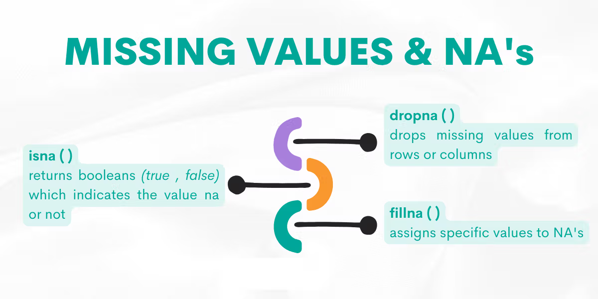
Function: dropna( )
This function helps us to remove NAs.
Syntax
The function’s syntax is:
DataFrame.dropna(*, axis=0, how=_NoDefault.no_default, thresh=_NoDefault.no_default, subset=None, inplace=False)By adding axis = 1, you will imply that you want to remove from columns or axis = 0 to remove from rows.
For a detailed explanation, please refer to the official Pandas documentation.
Example
Here is the question.
Find all businesses whose lowest and highest inspection scores are different. Output the corresponding business name and the lowest and highest scores of each business. HINT: you can assume there are no different businesses that share the same business name Order the result based on the business name in ascending order.
In this question, the city of San Francisco asks us to find all businesses whose lowest and highest scores are different.
To do that, we will first calculate the min and max by using the agg( ) function and rename the column to business_name afterward. Then we will filter the data by adding conditions where the highest and lowest scores can not be equal.
Now, in the last stage of our code, we will use the dropna( ) method to remove the NA values. By using it with equaling the inplace argument to true, we say that to transform the DataFrame.
Let’s see the code.
import pandas as pd
import numpy as np

ins_score = sf_restaurant_health_violations.groupby(['business_name'])['inspection_score'].agg(min_score = 'min', max_score = 'max').reset_index()
ins_score = ins_score.rename(columns={"": "business_name"})
result = ins_score[ins_score['min_score'] != ins_score['max_score']].sort_values('business_name')
result.dropna()
Here is the output.
| business_name | min_score | max_score |
|---|---|---|
| City Super | 77 | 78 |
| Fresca Gardens, Inc | 82 | 88 |
| Jiang Ling Cuisine Restaurant | 72 | 74 |
| Peet's Coffee & Tea | 94 | 96 |
| Project Juice | 96 | 100 |
| Roxanne Cafe | 86 | 92 |
| Sutter Pub and Restaurant | 88 | 90 |
| Wines of California Wine Bar | 88 | 92 |
Function: fillna( )
This function helps us replace the NA values with the custom ones.
Syntax
The function’s syntax is:
DataFrame.fillna(value=None, *, method=None, axis=None, inplace=False, limit=None, downcast=None)
You can fill the NA values with the value you include as an argument. Like many other Pandas functions, you can create a new DataFrame by setting an inplace argument to True or False.
For a detailed explanation, please refer to the official Pandas documentation.
Example
Here is the question.
Find the vintage years of all wines from the country of Macedonia. The year can be found in the 'title' column. Output the wine (i.e., the 'title') along with the year. The year should be a numeric or int data type.
The Wine Magazine asks us to find the vintage years of all wines from Macedonia.
First, we will select Macedonia by using conditions with bracket indexing. Then we will extract the year information from the title using the str( ) methods with the fillna( ) function.
Here we use the fillna( ) function with zero, meaning we will replace NAs with zeros. Then we will change its type to year and select the title and years afterward.
Now let’s see the code.
import pandas as pd
import numpy as np
macedonia = winemag_p2[winemag_p2['country'] == 'Macedonia']
macedonia['year'] = (macedonia['title'].str.extract('(\d{4,4})')).fillna(0).astype(int)
result = macedonia [['title','year']]
Here is the output.
| title | year |
|---|---|
| Macedon 2010 Pinot Noir (Tikves) | 2010 |
| Stobi 2011 Macedon Pinot Noir (Tikves) | 2011 |
| Stobi 2011 Veritas Vranec (Tikves) | 2011 |
| Bovin 2008 Chardonnay (Tikves) | 2008 |
| Stobi 2014 uilavka (Tikves) | 2014 |
Function: isna ()
It returns a Boolean and shows whether the value is NA.
Syntax
The function’s syntax is:
DataFrame.isna()For a detailed explanation, please refer to the official Pandas documentation.
Example
Here is the question.
Interview Question Date: May 2022
Write a query to get a list of products that have not had any sales. Output the ID and market name of these products.
In this question, Amazon asks us to find a list of products with no sales.
First, we will merge our two DataFrames on the right. When merging DataFrames, it will assign the NA to the non-matching values automatically.
Actually, the NA values are our answer because we want to find a product with no sales. After merging the DataFrames, the area that has the NAs will be the products with no sales.
To find the name of the market and the product id, we will use bracket indexing with the result.
Here is the code.
import pandas as pd
sales_and_products = fct_customer_sales.merge(dim_product, on='prod_sku_id', how='right')
result = sales_and_products[sales_and_products['order_id'].isna()][['prod_sku_id', 'market_name']]
Here is the output.
| prod_sku_id | market_name |
|---|---|
| P473 | Apply IPhone 13 Pro Max |
| P481 | Samsung Galaxy Tab A |
| P483 | Dell XPS13 |
| P488 | JBL Charge 5 |
Merging
Sometimes, to find an answer to your questions, you might need more than one DataFrame. Of course, there are multiple ways to merge them in Pandas. The next function in our Pandas cheat sheet is Merging. Let’s explore them by giving examples from the platform.

Function: concat( )
This function will be used to bond two DataFrames across their rows or columns
Syntax
The function’s syntax is:
pandas.concat(objs, *, axis=0, join='outer', ignore_index=False, keys=None, levels=None, names=None, verify_integrity=False, sort=False, copy=True)
For a detailed explanation, please refer to the official Pandas documentation.
Example
Here is the question.
Find all possible varieties which occur in either of the winemag datasets. Output unique variety values only. Sort records based on the variety in ascending order.
The Wine Magazine asks us to find all possible varieties which occur in either winemag dataset.
To do that, we first need to combine both data sets by selecting varieties first from both DataFrames and assigning them to two different DataFrames, p1 and p2.
Then, we will concatenate them across the columns by equaling the axis to zero. By equaling zero to the axis, we say to the function that we want to combine DataFrames along the indexes.
If we equate it to one, we want to combine DataFrames along the columns.
To find distinct values, we use drop_duplicates( ).
Let’s see the code.
import pandas as pd
import numpy as np

p1 = winemag_p1['variety']
p2 = winemag_p2['variety']
result = pd.concat([p1,p2],axis = 0).drop_duplicates()
Here is the output.
| variety |
|---|
| Merlot |
| Prosecco |
| Cabernet Sauvignon |
| Sauvignon Blanc |
| Rhone-style Red Blend |
Function: merge( )
This function combines two DataFrames on columns or indices.
Syntax
The function’s syntax is:
pandas.merge(left, right, how='inner', on=None, left_on=None, right_on=None, left_index=False, right_index=False, sort=False, suffixes=('_x', '_y'), copy=True, indicator=False, validate=None)For a detailed explanation, please refer to the official Pandas documentation.
Example
Here is the question.
Find the team division of each player. Output the player name along with the corresponding team division.
ESPN asks us to find the team division of each player.
To solve this problem, we will merge two DataFrames on the school name, which is the common element of both. Then we will select the player name and the division by using bracket indexing.
Let’s see the code.
import pandas as pd
import numpy as np
result = pd.merge(college_football_teams,college_football_players, on = 'school_name')[['player_name','division']]
Here is the output.
| player_name | division |
|---|---|
| Ralph Abernathy | FBS (Division I-A Teams) |
| Mekale McKay | FBS (Division I-A Teams) |
| Trenier Orr | FBS (Division I-A Teams) |
| Bennie Coney | FBS (Division I-A Teams) |
| Johnny Holton | FBS (Division I-A Teams) |
Function: join( )
It adds two DataFrames together on a key column or index.
Syntax
The function’s syntax is:
DataFrame.join(other, on=None, how='left', lsuffix='', rsuffix='', sort=False, validate=None)For a detailed explanation, please refer to the official Pandas documentation.
Example
Here is the question.
Interview Question Date: January 2021
Which company had the biggest month call decline from March to April 2020? Return the company_id and calls difference for the company with the highest decline.
Ring Central asks us to find the company with the biggest monthly decline in users placing a call from March to April 2020.
The output should contain the company id and calls variance for the company with the highest decline.
Now, to do that, we will use the merge( ) and join( ) functions to combine two DataFrames.
First, we merge DataFrames on user_id.
Then, we search for March and April by using the between( ) and groupby( ) functions to filter. What follows is using the count( ) function to find the number of calls and the to_frame( ) function to assign the result to the March and April DataFrames.
Lastly, we use the join( ) function with the March DataFrame to add it to April from the left. Since we use the left join, there will be NAs; that’s why we will fill them with zero by using the fillna( ) function, which we explained earlier.
Let’s see the code.
import pandas as pd

merged = pd.merge(rc_calls, rc_users, how='left', on='user_id')
march = merged[merged['date'].between('2020-04-01', '2020-04-30')].groupby(['company_id'])['call_id'].count().to_frame('apr_calls')
april = merged[merged['date'].between('2020-03-01', '2020-03-31')].groupby(['company_id'])['call_id'].count().to_frame('mar_calls')

result = march.join(april, how='left')
result['apr_calls'] = result['apr_calls'].fillna(0)
result['calls_var'] = result['mar_calls'] - result['apr_calls']
result[result['calls_var'] == result['calls_var'].max()][['calls_var']].reset_index()
Here is the output.
| company_id | calls_var |
|---|---|
| 3 | 2 |
Plotting
In Python, you have many library options to make visualizations, like Matplotlib, Plotly, or Seaborn. Yet, Panda has its own functions, and it also can work with Matplotlib. Let’s understand the next function ‘plotting’ in our Pandas cheat sheet.
Here is the official page of the Pandas plot.
We have many graph options like:
- line
- bar
- barh
- hist
- box
- kde
- density
- area
- pie
- scatter
- hexbin
We will go through some of them by creating a DataFrame and drawing a graph. Let’s draw a bar graph, line chart, pie chart, and scatter graph as an example.
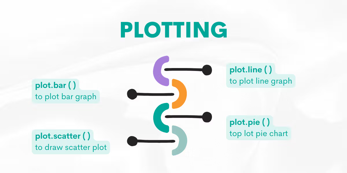
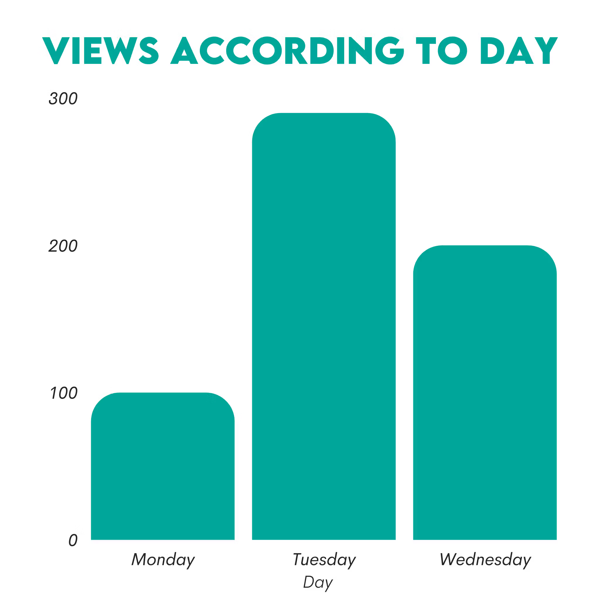
Function: plot.bar( )
Helps us to draw a bar plot.
Syntax
The function’s syntax is:
DataFrame.plot.bar(x=None, y=None, **kwargs)For a detailed explanation, please refer to the official Pandas documentation.
Example
Now, let’s first suppose we have a website and our views change according to day. We want to visualize this data.
First, we will create the DataFame containing days and views data.
Then we will draw a graph, setting x as days and y as views. Also, rot = 0 helps us to rotate the xticks (Monday, Tuesday, Wednesday).
Let’s see the code.
import pandas as pd
df = pd.DataFrame({'Day':['Monday', 'Tuesday', 'Wednesday'], 'views':[100, 300, 200]})
df.plot.bar(x='Day', y='views', rot=0, title = "Views According to Day")
Here is the output.

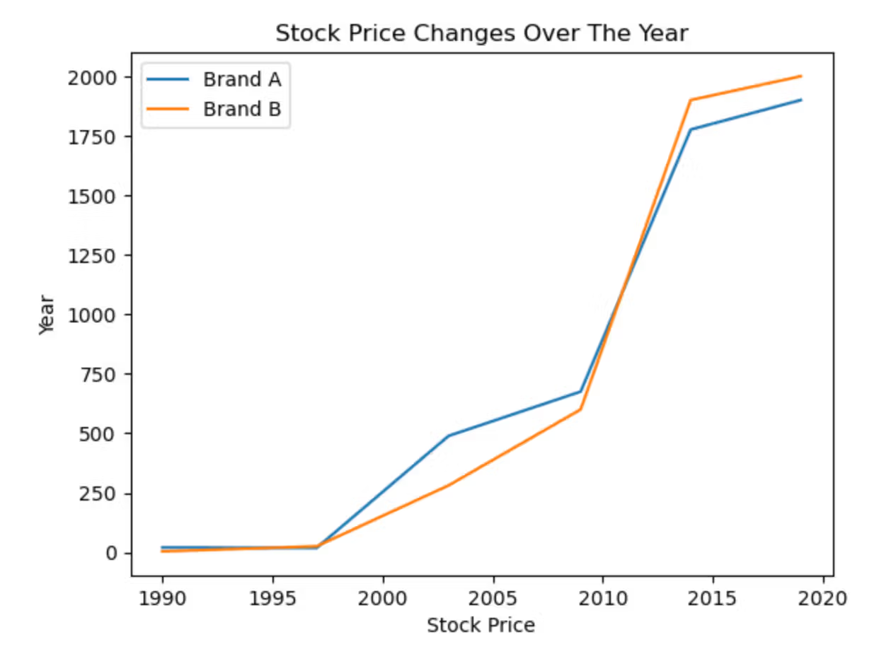
Function: plot.line( )
Helps us to draw a line plot.
Syntax
The function’s syntax is:
DataFrame.plot.line(x=None, y=None, **kwargs)For a detailed explanation, please refer to the official Pandas documentation.
Example
Here, we will draw the line graph. Suppose Brand A has the following stock prices; 20, 18, 489, 675, 1776, and 1900.
Also, Brand B has the following stock prices; 4, 25, 281, 600, 1900, and 2000.
The values are for the years between 1990 and 2020.
First, we will create DataFrame, and add years as an index. Then we will use the line function and add the title, xlabel, and ylabel as follows.
Let’s see the code.
import pandas as pd
df = pd.DataFrame({
   'Brand A': [20, 18, 489, 675, 1776, 1900],
   'Brand B': [4, 25, 281, 600, 1900, 2000]
   }, index=[1990, 1997, 2003, 2009, 2014, 2019])
lines = df.plot.line(title = "Stock Price Changes Over The Year", xlabel = "Stock Price", ylabel = "Year")
Here is the output.

Function: plot.pie( )
This plotting function is used for drawing a pie plot.
Syntax
The function’s syntax is:
DataFrame.plot.pie(**kwargs)For a detailed explanation, please refer to the official Pandas documentation.
Example
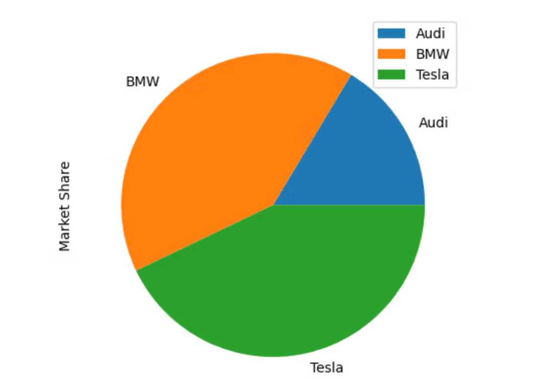
Now, the numbers we’ll use here are fictional. Let's draw a pie chart containing the market share of BMW, Audi, and Tesla
Market Shares are as follows.
- Audi: 2439.7
- BMW: 6051.8
- Tesla: 6378.1
First, we will create a DataFrame that shows the market share for each brand.
After that, we will create a pie chart and define y as a Market Share. Also, we defined figsize as (5,8), which are width, and height, respectively.
Let’s see the code.
import pandas as pd

df = pd.DataFrame({'Market Share': [2439.7, 6051.8, 6378.1]},
                  index=['Audi', 'BMW', 'Tesla'])
plot = df.plot.pie(y='Market Share', figsize=(5, 8))
Here is the output.

Function: plot.scatter( )
Helps us to draw a scatter plot.
Syntax
The function’s syntax is:
DataFrame.plot.scatter(x, y, s=None, c=None, **kwargs)For a detailed explanation, please refer to the official Pandas documentation.
Example
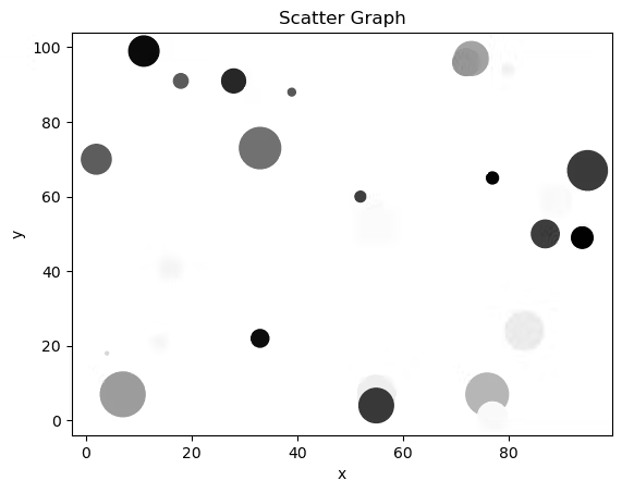
Here, we will draw a scatter graph.
First, we will define 30 different numbers between 1 and 100 as x and y by using the randint( ) function from NumPy.
Then, by using the rand( ) function from NumPy, we will create random numbers between 1 and 30. We will multiply the result by 30, square it, and assign it to the area.
And for the colors, we will again use the rand function from NumPy, create 30 different numbers between 0 to 100 and assign it to the colors.
Now, we will use our x and y and define the graph by equaling the title argument as a “Scatter Graph”. We will equal c (marker colors ) to the colors we already defined, which helps us give 30 different random numbers between 0 and 100 to each marker.
By doing that, each marker has its own unique colors.
After that, we will equal s (marker size) to the area. That assigns a unique area size, which we already calculated. By doing that, each marker now has its own unique size.
Let's see the code.
import pandas as pd
import numpy as np

x = np.random.randint(1,100, size = 30)
y = np.random.randint(1,100, size = 30)
df = pd.DataFrame({'x':x, 'y':y})

area = (30 * np.random.rand(30))**2
colors = np.random.rand(30)

df.plot.scatter('x', 'y', title = "Scatter Graph",c= colors, s =  area)
Here is the output.

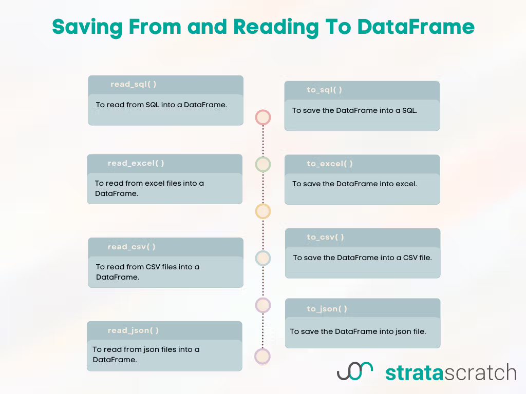
Saving From and Reading To DataFrame
Here’s the next function in our Pandas cheat sheet that you should know. Sometimes, you need to read data from other sources into a DataFrame or save it from DataFrame to different file types such as JSON, Excel, CSV, or SQL tables. These are the functions that will help you with this task.

Function: read_excel( )
To read from an excel file into a DataFrame.
Syntax
The function’s syntax is:
pandas.read_excel(io, sheet_name=0, *, header=0, names=None, index_col=None, usecols=None, squeeze=None, dtype=None, engine=None, converters=None, true_values=None, false_values=None, skiprows=None, nrows=None, na_values=None, keep_default_na=True, na_filter=True, verbose=False, parse_dates=False, date_parser=None, thousands=None, decimal='.', comment=None, skipfooter=0, convert_float=None, mangle_dupe_cols=True, storage_options=None)For a detailed explanation, please refer to the official Pandas documentation.
Example
Let’s see the code.
import pandas as pd

df = pd.read_excel(“path“)
If you want to read from an Excel sheet, you should specify the command like this.
import pandas as pd

df = pd.read_excel(“path“, sheet_name = “ “)
Function: to_excel( )
This function is used for saving your DataFrame as an Excel file in your working directory.
Syntax
The function’s syntax is:
DataFrame.to_excel(excel_writer, sheet_name='Sheet1', na_rep='', float_format=None, columns=None, header=True, index=True, index_label=None, startrow=0, startcol=0, engine=None, merge_cells=True, encoding=_NoDefault.no_default, inf_rep='inf', verbose=_NoDefault.no_default, freeze_panes=None, storage_options=None)
For a detailed explanation, please refer to the official Pandas documentation.
Example
Let’s see the code.
import pandas as pd

df1.to_excel(“output.xlsx”)
To save this excel file in the sheet, you can write the below code.
import pandas as pd

df1.to_excel(“output.xlsx”, sheet_name = “Sheet 1”)
Function: read_csv( )
This function is used to read from the CSV file into a DataFrame.
Syntax
The function’s syntax is:
pandas.read_csv(filepath_or_buffer, *, sep=_NoDefault.no_default, delimiter=None, header='infer', names=_NoDefault.no_default, index_col=None, usecols=None, squeeze=None, prefix=_NoDefault.no_default, mangle_dupe_cols=True, dtype=None, engine=None, converters=None, true_values=None, false_values=None, skipinitialspace=False, skiprows=None, skipfooter=0, nrows=None, na_values=None, keep_default_na=True, na_filter=True, verbose=False, skip_blank_lines=True, parse_dates=None, infer_datetime_format=False, keep_date_col=False, date_parser=None, dayfirst=False, cache_dates=True, iterator=False, chunksize=None, compression='infer', thousands=None, decimal='.', lineterminator=None, quotechar='"', quoting=0, doublequote=True, escapechar=None, comment=None, encoding=None, encoding_errors='strict', dialect=None, error_bad_lines=None, warn_bad_lines=None, on_bad_lines=None, delim_whitespace=False, low_memory=True, memory_map=False, float_precision=None, storage_options=None)
For a detailed explanation, please refer to the official Pandas documentation.
Example
Now, we will read from CSV in rotten_tomatoes_movies.csv files.
Let’s see the code.
import pandas as pd

df_movie = pd.read_csv('rotten_tomatoes_movies.csv')
Function: to_csv( )
If you want to save your DataFrame as CSV, here is the function for you.
Syntax
The function’s syntax is:
DataFrame.to_csv(path_or_buf=None, sep=',', na_rep='', float_format=None, columns=None, header=True, index=True, index_label=None, mode='w', encoding=None, compression='infer', quoting=None, quotechar='"', lineterminator=None, chunksize=None, date_format=None, doublequote=True, escapechar=None, decimal='.', errors='strict', storage_options=None)
For a detailed explanation, please refer to the official Pandas documentation.
Example
Let’s see the code.
import pandas as pd

df.to_csv(‘output.csv')
Also, you can save this file as a zip file containing output.csv.
Let’s see the code.
import pandas as pd

df.to_csv('output.zip',compression=compression_opts)
Function: read_json( )
This function reads JSON into a DataFrame.
Syntax
The function’s syntax is:
pandas.read_json(path_or_buf, *, orient=None, typ='frame', dtype=None, convert_axes=None, convert_dates=True, keep_default_dates=True, numpy=False, precise_float=False, date_unit=None, encoding=None, encoding_errors='strict', lines=False, chunksize=None, compression='infer', nrows=None, storage_options=None)For a detailed explanation, please refer to the official Pandas documentation.
Example
Let’s see the code.
import pandas as pd

df = pd.read_json('data.json')
Function: to_json( )
This function converts the object to a JSON string.
Syntax
The function’s syntax is:
DataFrame.to_json(path_or_buf=None, orient=None, date_format=None, double_precision=10, force_ascii=True, date_unit='ms', default_handler=None, lines=False, compression='infer', index=True, indent=None, storage_options=None)For a detailed explanation, please refer to the official Pandas documentation.
Example
Let’s see the code.
import pandas as pd

x = pd.to_json(“output”)
Function: read_sql( )
This function is used to read from SQL.
Syntax
The function’s syntax is:
pandas.read_sql(sql, con, index_col=None, coerce_float=True, params=None, parse_dates=None, columns=None, chunksize=None)
For a detailed explanation, please refer to the official Pandas documentation.
Example
To read data from SQL, you should first define a connection.
Let’s see the code.
import pandas as pd
from sqlite3 import connect
conn = connect(':memory:')

pd.read_sql('SELECT column, date FROM test_data', conn)
Function: to_sql( )
It write DataFrames to a SQL database.
If the same table exists, we will replace it by equaling the if_exists argument to “replace”.
Syntax
The function’s syntax is:
DataFrame.to_sql(name, con, schema=None, if_exists='fail', index=True, index_label=None, chunksize=None, dtype=None, method=None)
For a detailed explanation, please refer to the official Pandas documentation.
Example
Let’s see the code.
import pandas as pd

df.to_sql(‘users’, con, if_exists='replace')
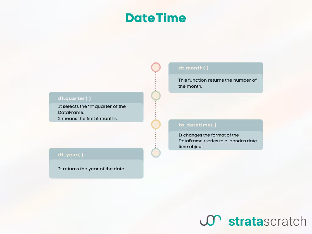
DateTime
When working with different data types like DateTime, there might be several type-specific functions. In Pandas, there are many functions for manipulating DateTime.
The next, in our Pandas cheat sheet, we will examine these by giving examples from the platform.
Function: dt.month( )
It returns the number of the month. Meaning January will equal 1.
Syntax
The function’s syntax is:
Series.dt.month
For a detailed explanation, please refer to the official Pandas documentation.
Example
Here is the question.
Interview Question Date: June 2021
Find the total monetary value for completed orders by service type for every month. Output your result as a pivot table where there is a column for month and columns for each service type.
In this question, Uber asks us to find the total monetary value for completed orders by service type for every month. The output should contain the month and each service type.
Now, we will select the completed order by using conditions with bracket indexing. Then we will add the month column by applying the dt.month( ) function to the order date.
Let’s see the code.
import pandas as pd
import numpy as np
result = uber_orders[uber_orders['status_of_order'] == 'Completed']
result['month'] = pd.to_datetime(uber_orders['order_date']).dt.month
result = pd.pivot_table(result, values='monetary_value', index=['month'],
                columns=['service_name'], aggfunc=np.sum).reset_index()
Here is the output.
| month | Uber_BOX | Uber_CLEAN | Uber_FOOD | Uber_GLAM | Uber_KILAT | Uber_MART | Uber_MASSAGE | Uber_RIDE | Uber_SEND | Uber_SHOP | Uber_TIX |
|---|---|---|---|---|---|---|---|---|---|---|---|
| 1 | 7549106565 | 704727660 | 39263369600 | 307227375 | 34616400 | 1009881600 | 2344439370 | 198876603380 | 32917462760 | 13492215100 | 1442579 |
| 2 | 7471476791 | 620599980 | 34245493100 | 354183830 | 108735900 | 839493200 | 2337281310 | 213629295880 | 37539087040 | 10231901680 | 49598995 |
| 3 | 8970977198 | 846946100 | 36464276394 | 441279020 | 209718600 | 871161200 | 2849679560 | 237234890620 | 41087692100 | 9524369400 | 12487285 |
| 4 | 434948059 | 32323200 | 1214895500 | 17927910 | 11930100 | 29338400 | 99745100 | 9636040960 | 1700529740 | 342647760 | 294158 |
Function: dt.quarter( )
It returns a specified number of quarters from the data.
Syntax
The function’s syntax is:
Series.dt.quarterFor a detailed explanation, please refer to the official Pandas documentation.
Example
Here is the question.
Interview Question Date: September 2021
How many searches were there in the second quarter of 2021?
Meta asks us the calculate the searches in the second quarter of 2021.
Let’s first find the second quarter by selecting the date and using our dt.quarter( ) function.
Then we will use this in the Facebook searches to find the searches of the second quarter. After that, we will add another filter used to select 2021 year.
Next, we will select the searches in 2021. To find their count, let’s use the result in the len( ) function and assign it to the result variable.
Let’s see the code.
import pandas as pd

searches_in_q2 = fb_searches[(fb_searches['date'].dt.quarter == 2) & (fb_searches['date'].dt.year == 2021)]
result = len(searches_in_q2)
Here is the output.
Function: to_datetime( )
It turns the series or DataFrames into a Pandas DateTime object.
Syntax
The function’s syntax is:
pandas.to_datetime(arg, errors='raise', dayfirst=False, yearfirst=False, utc=None, format=None, exact=True, unit=None, infer_datetime_format=False, origin='unix', cache=True)For a detailed explanation, please refer to the official Pandas documentation.
Example
Here is the question.
Interview Question Date: July 2021
Find the monthly active users for January 2021 for each account. Your output should have account_id and the monthly count for that account.
Salesforce asks us to find each account's monthly active users for January 2021.
First, we will use the to_datetime( ) function to change the DataFrame format. We will select the date column with an index bracket, then equal it to the to_datetime function. We will first define our date column as an argument, then use the format argument by equaling it %Y-%m-%d. That helps us to change our date column order to Year, Month, and Date, respectively.
After that, we will use the dt.year( ) function to select the year and the dt.month( ) function to select the month. Then we will use the groupby( ) function with the nunique( ) function to find the distinct values and reset the index afterward to remove indexes the groupby( ) added.
Let’s see the code.
import pandas as pd

df = sf_events
df['date'] = pd.to_datetime(df['date'],format='%Y-%m-%d')
result = df[(df['date'].dt.year == 2021) & (df['date'].dt.month == 1)].groupby('account_id')['user_id'].nunique().reset_index()
Here is the output.
| account_id | user_id |
|---|---|
| A1 | 3 |
| A2 | 2 |
| A3 | 1 |
Function: dt_year( )
It returns the year from the data.
Syntax
The function’s syntax is:
Series.dt.year
For a detailed explanation, please refer to the official Pandas documentation.
Example
Here is the question.
Interview Question Date: August 2022
Calculate the sales revenue for the year 2021.
In this problem, Amazon asks us to calculate the sales revenue for the year 2021.
First, we will select the year by using the dt.year( ) function and use the result to find the 2021 year in our DataFrame. Then we use the sum( ) function to calculate the sales.
Let’s see the code.
import pandas as pd

result = amazon_sales[amazon_sales['order_date'].dt.year == 2021]['order_total'].sum()
Here is the output.
This one is our last example in that article. If you want more, here are Pandas Interview Questions.
Summary
In this Pandas cheat sheet, you learned about Pandas features in the interview questions by the companies such as Meta, Google, Amazon, and Forbes.
For more examples, here are Python Coding Interview Questions.
These questions showed you how to explore, merge, and operate DataFrames, find specific values, and locate missing ones.
Also, you learned reading and writing from different data types to the different data types, like csv, xlslx.
Finally, we also mentioned data visualization with Pandas.
You can start preparing for interviews by practicing related interview questions today. Here are Python Interview Questions and Answers.
To be successful in interviews, you should develop a habit. To do that, join the StrataScratch community and sign up today to help us find your dream job.
Latest Posts:


Share