Python Window Functions

Categories:
 Written by:
Abhishek Ramesh
This article focuses on different types of Python window functions, where and how to implement them, practice questions, reference articles and documentation.
Window function is a popular technique used to analyze a subset with related values. It is commonly used in SQL, however, these functions are extremely useful in Python as well.
If you would like to check out our content on SQL Window Functions, we have also created an article "The Ultimate Guide to SQL Window Functions" and a YouTube video!
This article discusses:
- Different types of window functions
- Where / How to implement these functions
- Practice Questions
- Reference articles / Documentation
A general format is written for each of these functions for you to understand and implement on your own. The format will include bold italicized text which indicate these are the sections of the function you need to replace during implementation.
For example:
dataframe.groupby(level='groupby_column').agg({‘aggregate_column’: ‘aggregate_function’})
Texts such as 'dataframe' and 'groupby_column' are bold and italicized meaning you should replace them with the actual variables.
Texts such as ‘.groupby’ and ‘level’ which are not bold and italicized are required to remain the same to execute the function.
Let’s suppose Amazon asks to find the total cost each user spent on their amazon orders.
An implementation of this function this dataset would look similar to this:
amazon_orders.groupby(level='user_id').agg({'cost': 'sum'})
Table of Contents
- Python Window Functions overview diagram
- Aggregate
- Group by
- Rolling
- Expanding
- Ranking
- Row number
- reset_index()
- cumcount()
- Rank
- default_rank
- min_rank
- NA_bottom
- descending
- Dense rank
- Percent rank
- N-Tile / qcut()
- Row number
- Value
- Lag / Lead
- First / Last / nth value
Functions
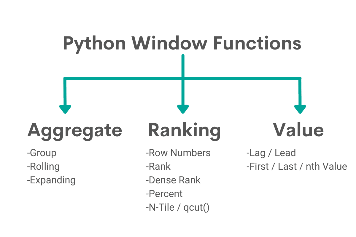
While there is not any official classification of Python window functions, these are the common functions implemented.
Aggregate

These are some common types of aggregate functions
- Average
- Max
- Min
- Sum
- Count
Each of these aggregate functions (except count which will be explained later) can be used in three types of situations
- Group by
- Rolling
- Expanding
Example
- Group by: Facebook is trying to find the average revenue of Instagram for each year.
- Rolling: Facebook is trying to find the rolling 3 year average revenue of Instagram
- Expanding: Facebook is trying to find the cumulative average revenue of Instagram with an initial size of 2 years.
Group by
Group by aggregates is computing a certain column by a statistical function within each group. For example in a dataset
Let’s use a question from Amazon to explain this topic. This question is asking us to calculate the percentage of the total expenditure a customer spent on each order. Output the customer’s first name, order details (product name), and percentage of the order cost to their total spend across all orders.
Remember when approaching questions follow the 3 steps
- Ask clarifying questions
- State assumptions
- Attempt the question
When approaching these questions, understand which columns need to be grouped and which columns need to be aggregated.
For the Amazon example,
Group by: customer first_name, order_id, order_details
Aggregate: total_order_cost
In this question, there are 2 tables which need to be joined to get the customer’s first name, item, and spending. After merging both tables and filtering to get the required columns, to get the following dataset
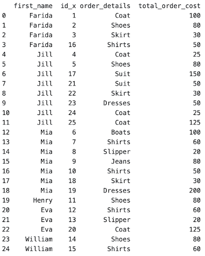
Once necessary data is set in a single table, it is easier to manipulate.
Here we can find the total spending by person by grouping first_name and sum of total_order_cost
This is a general format on how to group by and aggregate the required columns.
dataframe.groupby(level='groupby_column').agg({'aggregate_column': 'aggregate_function'})
In reference to the Amazon example, this is the executing code.
total_spending = customer_orders.groupby("first_name").agg({'total_order_cost' : 'sum'})This code will output the following dataframe
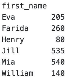
After this, we want to add a column to the merged data frame to represent total spending by each person.
Let’s join both dataframes on the person’s first_name
pd.merge(merged_dataframe, total_spending, how="left", on="first_name")Now we get the following dataset
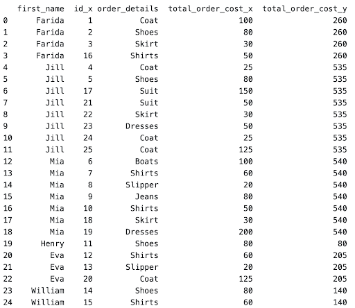
As seen, the total_order_cost_y column represents the total spending per person and the total_order_cost_x to represent the cost per order. After this, this is a simple division of 2 columns to create the percentage of the spending column AND filtering the output to get the required columns.
result = df3[["first_name", "order_details", "percentage_total_cost"]]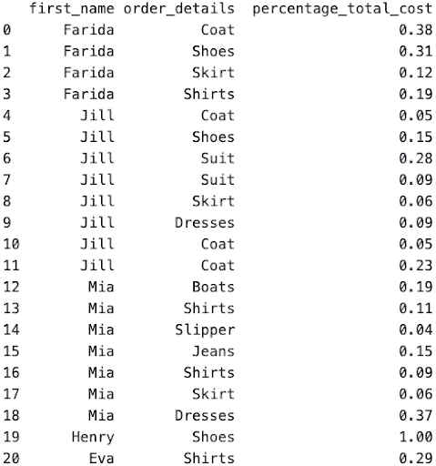
However for certain situations, it is required to sort the values within each group. This is where the sort_values() function is implemented.
Referencing the amazon question example:
Suppose the interviewer asks to order the percentage_total_cost in descending order by person.
result = result.sort_values(by=['first_name', 'percentage_total_cost'], ascending = (True, False))- The dataset has already been loaded as a pandas.DataFrame.
- print() functions and the last line of code will be displayed in the output.
- In order for your solution to be accepted, your solution should be located on the last line of the editor and match the expected output data type listed in the question.
Practice
- https://platform.stratascratch.com/coding/9711-facilities-with-lots-of-inspections?python=
- https://platform.stratascratch.com/coding/9899-percentage-of-total-spend?python=1
- https://platform.stratascratch.com/coding/2044-most-senior-junior-employee?python=1
Reference
Rolling vs Expanding Function
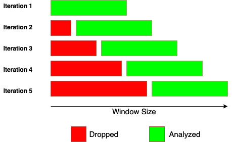
Before diving into how to execute a rolling or expanding function, let’s understand how each of these functions works. While rolling function and expanding function work similarly, there is a significant difference in the window size. Rolling function has a fixed window size, while the expanding function has a variable window size.
These images explain the difference between rolling and expanding functions.
Rolling Function
Expanding Function
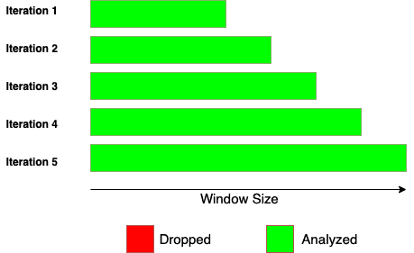
Rolling and expanding functions both start with the same window size, but expanding function incorporates all the subsequent values beyond the initial window size.
Example: AccuWeather, a weather forecasting company, is trying to find the rolling and expanding average 10 day weather of San Francisco in January.
Rolling: Starting with a window size of 10, we take the average temperature from January 1st to January 10th. Next we take January 2nd to January 11th and so on. This shows the window size in rolling functions remains the same.
Expanding: Starting with a window size of 10, we take the average temperature from january 1st to January 10th. However, next we’ll take the average temperature from January 1st to January 11th. Then, January 1st to January 12th and so on. Therefore the window size has “expanded”.
While there are many aggregate functions that can be used in rolling/expanding functions, this article will discuss the frequently used functions (sum, average, max, min).
This brings us to the reason why the count function is not used in rolling and expanding functions. Count is used when a certain variable is grouped and there is a need to count the occurrence of a value. In the rolling and expanding function, there is no grouping of rows, but a calculation on a specific column.
Rolling Aggregate
Implementation of rolling functions are straightforward.
A general format:
DataSeries.rolling(window_size).aggregate_function()
Example:
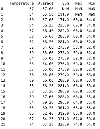
Temperature of San Francisco of the first 22 days of 2021. Let’s find the average, sum, maximum, and minimum of a 5 day rolling time period.
weather['Average'] = weather['Temperature'].rolling(5).mean()
weather['Sum'] = weather['Temperature'].rolling(5).sum()
weather['Max'] = weather['Temperature'].rolling(5).max()
weather['Min'] = weather['Temperature'].rolling(5).min()
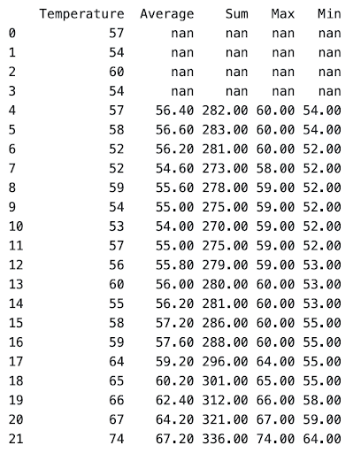
After row 4, the rolling function over a fixed window size of 5 calculates the average, sum, max, and min over the Temperature values. This means that in the average column in row 16, calculates the average of rows 12, 13, 14, 15, and 16.
As expected, the first 4 values of the rolling function columns are null due to not having enough values to calculate. Sometimes you still want to calculate the aggregate of the first n rows even if it doesn’t fit the number of required rows.
In that case, we have to set a minimum number of observations to start calculating. Within the rolling function, you can specify the min_periods.
DataSeries.rolling(window_size, min_periods=minimum_observations).aggregate_function()
weather['Average'] = weather['Temperature'].rolling(5, min_periods=1).mean()
weather['Sum'] = weather['Temperature'].rolling(5, min_periods=2).sum()
weather['Max'] = weather['Temperature'].rolling(5, min_periods=3).max()
weather['Min'] = weather['Temperature'].rolling(5, min_periods=3).min()
Practice
Reference
- https://pandas.pydata.org/docs/reference/api/pandas.DataFrame.rolling.html
- https://towardsdatascience.com/dont-miss-out-on-rolling-window-functions-in-pandas-850b817131db
Expanding Aggregate
Expanding function has a similar implementation to rolling functions.
DataSeries.expanding(minimum_observations).aggregate_function()
It is important to remember that unlike the rolling function, the expanding function does not set a window size, due to its variability. The minimum_observations is specified, so for rows less than the minimum_observations will be set as null.
Let’s use the same San Francisco Temperature example to explain expanding function
weather['Average'] = weather['Temperature'].expanding(5).mean()
weather['Sum'] = weather['Temperature'].expanding(5).sum()
weather['Max'] = weather['Temperature'].expanding(5).max()
weather['Min'] = weather['Temperature'].expanding(5).min()
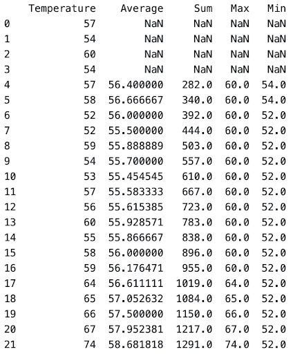
As it can be seen through the minimum temperature column, it takes the minimum value throughout the dataset, since it’s expanding beyond the minimum observations set.
- The dataset has already been loaded as a pandas.DataFrame.
- print() functions and the last line of code will be displayed in the output.
- In order for your solution to be accepted, your solution should be located on the last line of the editor and match the expected output data type listed in the question.
Reference
- https://pandas.pydata.org/docs/reference/api/pandas.DataFrame.expanding.html
- https://towardsdatascience.com/window-functions-in-pandas-eaece0421f7
- https://campus.datacamp.com/courses/manipulating-time-series-data-in-python/window-functions-rolling-expanding-metrics?ex=5
Ranking

Row Number
Counting the number of rows can be executed in 2 different situations each with a different function
- Across the entire dataframe - reset_index()
- Within groups - cumcount()
These are the equivalent functions as row_number() in SQL
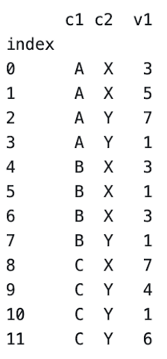
Let’s use the following sample dataset to explain both concepts
Reset_index
Within a dataframe, reset_index() will output the row number of each row.
General format to follow:
dataframe.reset_index()
To extract the nth row implement the .iloc() function
Dataframe.iloc[nth_row]
cumcount()
To calculate the row number within groups of a dataframe, you have to implement the cumcount() function in the following format
dataframe.groupby([‘column_names’]).cumcount()
Also remember to start the row count from 1 instead of the default 0, you need to add +1 to the cumcount() function
For the sample dataset, the implementation would be
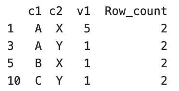
df['Row_count'] = df.groupby(['c1', 'c2']).cumcount()+1This would be the output
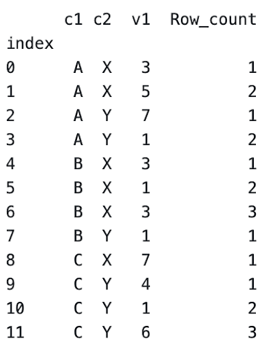
Now that you have the row_count within each group, sometimes you have to extract a specific index row of each group.
For example, the company asks to extract the 2nd indexed value within each group. We can extract this by returning each row with a row_count value of 2.
Using iloc again, we can extract the subset with the following general format
Dataframe.loc[dataframe[column_name] == index]
For the column dataset above, we would use
df.loc[df['Row_count'] == 2]to get the subset
- The dataset has already been loaded as a pandas.DataFrame.
- print() functions and the last line of code will be displayed in the output.
- In order for your solution to be accepted, your solution should be located on the last line of the editor and match the expected output data type listed in the question.
Questions:
- https://platform.stratascratch.com/coding/2004-number-of-comments-per-user-in-past-30-days?python=1
- https://platform.stratascratch.com/coding/9716-top-3-facilities?python=1
- https://platform.stratascratch.com/coding/10351-activity-rank?python=1
Reference:
- https://pandas.pydata.org/docs/reference/api/pandas.DataFrame.reset_index.html
- https://pandas.pydata.org/docs/reference/api/pandas.core.groupby.GroupBy.cumcount.html
Rank
Ranking functions as the name states ranks values based on a certain variable. Ranking function works slightly differently than its SQL equivalent.
Rank() function can be executed with the following general format
dataframe[column_name].rank()
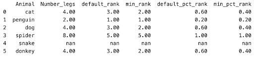
Let’s assume the following dataset from the Pandas ranking documentation.
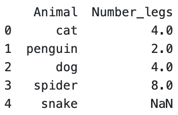
And create 4 new columns which both use the rank() function to explain the function and its most popular parameters better
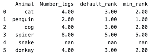
animal_legs['default_rank'] = animal_legs['Number_legs'].rank()
animal_legs['min_rank'] = animal_legs['Number_legs'].rank(method='min')
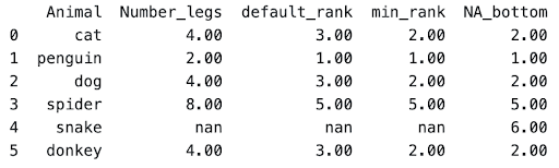
animal_legs['NA_bottom'] = animal_legs['Number_legs'].rank(method='min', na_option='bottom')
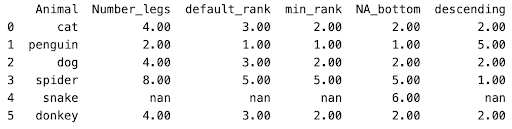
animal_legs['descending'] = animal_legs['Number_legs'].rank(method='min', ascending = False)
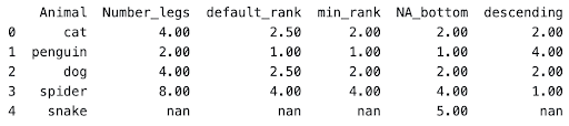
In this function we’re ranking the number_legs for each animal.
Let’s understand what each of the columns represents.
‘default_rank’
In a default rank() function, there are 3 important things to note.
- Ascending order is assumed true
- Null values are not ranked and left as null
- If n values are equal, the rank split is averaged between the values.
The n values rank splitting is a bit confusing, so let’s dive more into this to explain it better.
In SQL for the dataset above, since both cat and dog both have 4 legs, it would assume both as rank = 2 and spider with the next highest number of legs would have a rank of 4.
Instead of that, Pandas averages out the ‘would have been’ ranks between cat and dog.
There should be a rank of 2 and 3, but since cat and dog have the same value, the rank is the average of 2 and 3, which is 2.5
Let’s alter the animal's example to include ‘donkey’ which has 4 legs.
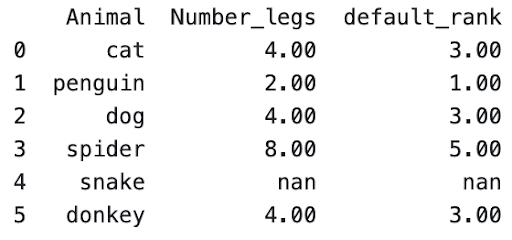
Penguin has the least number of legs with 2, so it has a rank = 1.
Since cat, dog, and donkey all have the next highest count of 4 legs, it will take the average of 2,3,4, due to 3 animals with the same value.
If we have 4 animals all with 4 legs, it will take the average of 2,3,4,5 = 3.5
‘min_rank’
When setting the parameter method=’min, instead of taking the average ranked value, it will take the minimum rank between equal values.
The minimum rank is the same as how the rank function in SQL works.
Using the animals example, the rank between dog and cat will now be 2 instead of 2.5.
And for the example with donkey, it will still assume a rank of 2, while spider will be set to a rank of 5.
‘NA_bottom’
Certain rows contain null values and under default conditions, the rank will also be set as null. In certain cases you would want the null values to rank the lowest or highest.
Setting the na_option as bottom would give the highest ranked value and setting as top would give it the lowest ranked value
In the animals example, we set null values as bottom and rank method as minimum
‘descending’
If you want to set the rank in descending order, set the parameter ascending as false.
Referring to the animals example, we set ascending to false and method as minimum
Questions:
- https://platform.stratascratch.com/coding/10169-highest-total-miles?python=
- https://platform.stratascratch.com/coding/10324-distances-traveled?python=
- https://platform.stratascratch.com/coding/2070-top-three-classes?python=1
Reference:
Dense Rank
Dense rank is similar to a normal rank with a slight difference.
During a normal rank function, ranking numbers may be skipped, while dense_rank doesn’t skip.
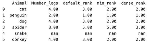
For example in the animals dataframe, after [dog, cat, donkey], spider was the next value. In minimum rank, it sets spiders as rank = 5, since 2,3,4 are technically set for cat,dog, and donkey.
In a dense rank, it will set the immediate consecutive ranks as seen above. Instead of 5th rank, spider was set to 3rd rank in dense_rank.
Fortunately, you just have to edit the method parameter in a rank function to get the dense rank
animal_legs['dense_rank'] = animal_legs['Number_legs'].rank(method='dense')All the other parameters, such as na_option and ascending, can also be set alongside the dense method as mentioned before.
Questions:
- https://platform.stratascratch.com/coding/9701-3rd-most-reported-health-issues?python=1
- https://platform.stratascratch.com/coding/2026-bottom-2-companies-by-mobile-usage
- https://platform.stratascratch.com/coding/2019-top-2-users-with-most-calls?python=1
Reference:
- https://pandas.pydata.org/docs/reference/api/pandas.DataFrame.rank.html
- https://dfrieds.com/data-analysis/rank-method-python-pandas.html
Percent rank (Percentile)
Percent rank is just a representation of the ranks compared to the highest rank.
As seen in the animals dataframe above, spider has a rank of 5 for both default_rank and min_rank. Since 5 is the highest rank, the other values would be compared to this.
For cat in default_rank, it has a value of 3, and 3 / 5 = 0.6 for default_pct_rank
For cat in min_rank, it has a value of 2, and 2 / 5 = 0.4 for min_pct_rank
Percentage rank is boolean parameter which can be set
animal_legs['min_pct_rank'] = animal_legs['Number_legs'].rank(method='min', pct=True)Questions:
- https://platform.stratascratch.com/coding/10303-top-percentile-fraud?python=1
- https://platform.stratascratch.com/coding/9611-find-the-80th-percentile-of-hours-studied?python=1
Reference:
- https://pandas.pydata.org/docs/reference/api/pandas.DataFrame.rank.html
- https://dfrieds.com/data-analysis/rank-method-python-pandas.html
- The dataset has already been loaded as a pandas.DataFrame.
- print() functions and the last line of code will be displayed in the output.
- In order for your solution to be accepted, your solution should be located on the last line of the editor and match the expected output data type listed in the question.
N-Tile / qcut()
qcut() is not a popular function, since ranking based on quantiles beyond percentiles are not as common. While it isn’t as popular, it is still an extremely powerful function!
If you don’t know the relationship between quantiles and percentiles, check out this article by statology!
Let’s take a question from DoorDash, to explain how qcut is used.
The question asks us to find the bottom 2% of the dataset, which is the first quantile from a 50-quantile split.
A general format to follow when using qcut():
pd.qcut(dataseries, q=number_quantiles, labels = range(lower_bound, upper_bound))
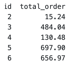
This is a subset of the dataset which we will use to analyze the usage of the qcut() function.
- dataseries → The column to analyze, which is total_order in this example
- number_quantiles → Number of quantiles to split by, which is 50 due to 50-quantile split
- labels → Range of ntiles, which 1-50 in this case. However, the upper bound is calculated as n-1. So if we set a range of 1-50, the highest ntile will be 49 instead of 50. Due to this, we set our upper bound as n+1, which in this example would be range(1,51)
For this example, this would be the following code.
result[‘ntile’] = pd.qcut(result['total_order'],q=50, labels=range(1, 50))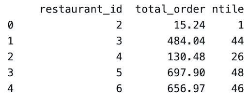
As seen in the example, ‘ntile’ has been split and represents the quantile.
It must also be noted that if the label range is not specified, the quantile range is returned.
For example executing the same code above without the labels range:
result[‘ntile_range’] = pd.qcut(result['total_order'],q=50) 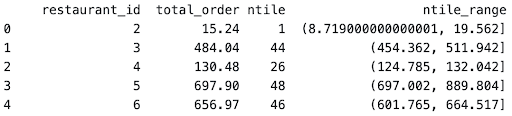
- The dataset has already been loaded as a pandas.DataFrame.
- print() functions and the last line of code will be displayed in the output.
- In order for your solution to be accepted, your solution should be located on the last line of the editor and match the expected output data type listed in the question.
Questions:
- qcut() → https://platform.stratascratch.com/coding/2036-lowest-revenue-generated-restaurants?python=1
Reference:
- https://pandas.pydata.org/docs/reference/api/pandas.qcut.html
- https://towardsdatascience.com/all-pandas-qcut-you-should-know-for-binning-numerical-data-based-on-sample-quantiles-c8b13a8ed844
Value
Lag / Lead
Lag and Lead functions are used to represent another column but are shifted by a single or multiple rows.
Let’s use a dataset given by Facebook (Meta) which represents the total cost of orders by each month.
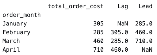
In the ‘Lag’ column, we can see that values were shifted down by one. 305 which is the total_order_cost for January, appears in the ‘Lag’ column but on the same row as February.
In the ‘Lead’ column, the opposite occurs. Rows are shifted up by one, so 285 which is the total_order_cost for February appears in the ‘Lead’ column in January.
This makes it easier to calculate comparing values side by side such as growth of sales by month.
A general format to follow:
dataframe[‘shifting_column’].shift(number_shift)
Code used for the data:
orders['Lag'] = orders['total_order_cost'].shift(1)
orders['Lead'] = orders['total_order_cost'].shift(-1)
Also another key point to remember is the null values that are present due to the shift. As seen there are 1 null values (NaN) in the Lag and Lead column, since the values have been shifted by 1. There will be n rows of null values, due to the data series being shifted by n rows. So for the first n rows of ‘Lag’ column and last n rows of ‘Lead’ column will be null values.
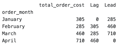
If you want to replace the null values that are generated by the shift, you can use the fill_value parameter.
We execute the code with updated parameters
orders['Lag'] = orders['total_order_cost'].shift(1, fill_value = 0)
orders['Lead'] = orders['total_order_cost'].shift(-1, fill_value = 0)
To get this as the output
- The dataset has already been loaded as a pandas.DataFrame.
- print() functions and the last line of code will be displayed in the output.
- In order for your solution to be accepted, your solution should be located on the last line of the editor and match the expected output data type listed in the question.
Questions:
- https://platform.stratascratch.com/coding/9637-growth-of-airbnb?python=
- https://platform.stratascratch.com/coding/9714-dates-of-inspection?python=
- https://platform.stratascratch.com/coding/2045-days-without-hiringtermination?python=1
Reference:
First/Last/nth value
Finding the nth value (including first and last) within groups of a dataset is fairly simple with Python as well.
Let’s use the same orders dataset by Facebook used in the Lag/Lead section.
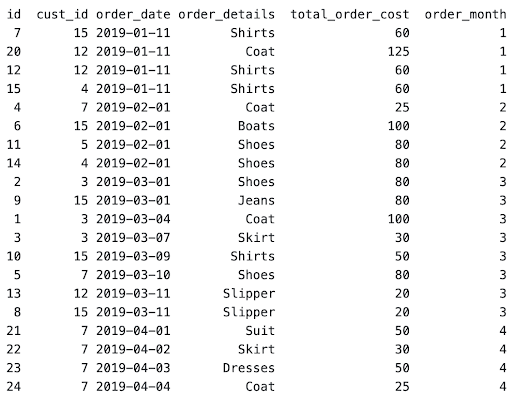
As seen here, the order_date has been ordered from earliest to latest.
Let’s find the first order of each month using the nth() function
General format:
dataframe.groupby(‘groupby_column’).nth(nth_value)
nth_value represents the indexed value
nth_value in the nth() function works the same way as extracting the nth_value in a list.
0 represents the first value
-1 represents the last value
Using the following code:
orders.groupby('order_month').nth(0)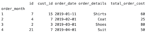
To return only a specific column, such as total_order_cost, you can specify this as well.
orders.groupby('order_month').nth(0)['total_order_cost'].reset_index()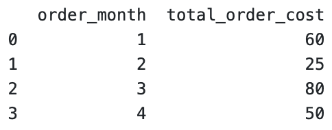
Now if you want to join the nth value to the respective grouped by columns in the original dataframe, you could use a merge function, similar to how the merge function was applied in the aggregate functions mentioned above. Make sure you remember to extract the column to merge on as well! In this example, it would be the ‘order_month’ index column, where you should use the reset_index() function.
- The dataset has already been loaded as a pandas.DataFrame.
- print() functions and the last line of code will be displayed in the output.
- In order for your solution to be accepted, your solution should be located on the last line of the editor and match the expected output data type listed in the question.
Reference:
- https://pandas.pydata.org/docs/reference/api/pandas.core.groupby.GroupBy.nth.html
Practice Questions Compiled
Aggregate
- Group by
- Rolling
- Expanding
- [[[ No Questions ]]]
Ranking
- Row_number()
- rank()
- dense_rank()
- percent_rank()
- ntile() / qcut()
Value
Share