NumPy for Data Science Interviews: Part 02

Part 2 of the series on NumPy for Data Science

In the previous article, we looked at the basics of using NumPy. We discussed

• The need for NumPy and comparison of NumPy array with Python lists and Pandas Series.
• Array attributes like dimensions, shape, etc.
• Special Arrays in NumPy
• Reshaping NumPy arrays
• Indexing and Slicing NumPy arrays
• Boolean Masks in NumPy arrays
• Basic Functions in NumPy
• Vectorized Operations

In the second part of the series, we move to advanced topics in NumPy and their application in Data Science. We will be looking at

• Random Number Generation
• Advanced Array operations
• Handling Missing Values
• Sorting and Searching functions in NumPy
• Broadcasting
• Matrix Operations and Linear Algebra
• Polynomials
• Curve Fitting
• Importing Data into and Exporting Data out of NumPy

If you have not worked with NumPy earlier, we recommend reading the first part of the NumPy series to get started with NumPy concepts.

Advanced Usage of NumPy

Random Number Operations with NumPy

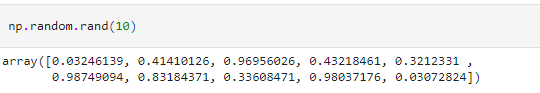
Random number generation forms a critical basis for scientific libraries. NumPy supports the generation of random numbers using the random() module. One of the simplest random number generating methods is rand(). The rand method returns a result from a uniform random distribution between zero and one.

We can specify the number of random numbers that we need to generate.

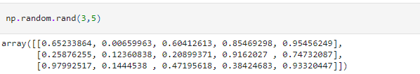
Or specify the shape of the resulting array. For example, in this case, we get fifteen uniformly distributed random numbers in the shape 3 x 5

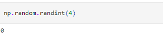
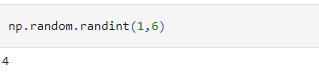
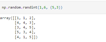
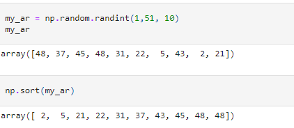
We can also generate integers in a specified range. For this, we use the randint() method.

We can also specify how many integers we want.

as with the rand method, in the randint function too, we can specify the shape of the final array

Sampling

We can also use random number generators to sample a given set population. For example, if we want to choose three colors out of 10 different colors, we can use the choice option.

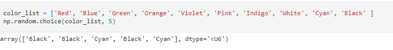
we can also specify if we want the choice to be repeated or not

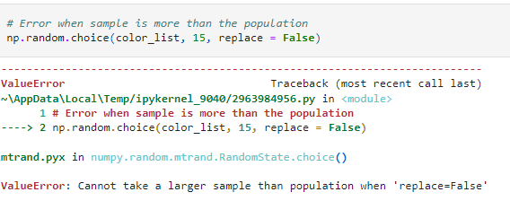
As you would expect, if the number of selections is more than the number of choices available, the function will return an error.

“Freezing” a Random State

A critical requirement in the Data Science world is the repeatability of results. While we choose random numbers to compute results, to be able to reproduce identical results, we need the same sequence of random numbers. To do this, we need to understand how random numbers are generated.

Most random numbers generated by computer algorithms are called pseudo-random numbers. In simple terms, these are a sequence of numbers that have the same property of random numbers but eventually repeat a pattern because of constraints like memory, disk space, etc. The algorithms use a start value called the seed to generate random numbers. A particular seed to an algorithm will output the same sequence of random numbers. Think of it as the registration number of a vehicle or the social security number. This number can be used to identify the sequence.

To reproduce the same set of random numbers, we need to specify the seed to the sequence. In NumPy, this can be achieved by setting the RandomState of the generator. Let us illustrate this with the following example. We had earlier chosen five colors from ten choices. Each time we execute the code, we may get different results. However, if we fix the RandomState before invoking the choice method, we will get the same result no matter how many times we execute the cell.

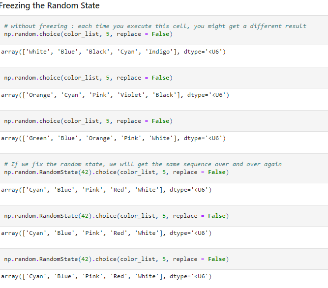
This is very helpful in data science operations like splitting a data set into training and testing data sets. You will find these seeding options in almost all sampling methods - sample, shuffle methods in Pandas, train_test_split method in scikit_learn et al.

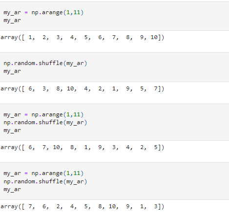
Another useful random number operation is shuffle. As the name suggests, the shuffle method well reorders an array’s elements.

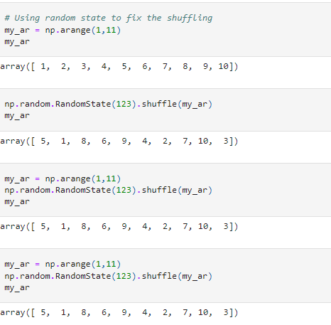
The shuffling results can also be “fixed” by specifying a RandomState().

Array Operations

NumPy supports a range of array manipulation operations. We had seen some basic ones in the first part of the NumPy series. Let us look at some advanced operations.

Splitting an Array.
We have a wide range of options to break the array in smaller arrays.

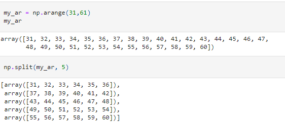
split()
The split method offers two major ways of splitting an array.
If we pass an integer, the array is split into equal-sized arrays.

It will return an error if the array cannot be divided into equal-sized sub-arrays.

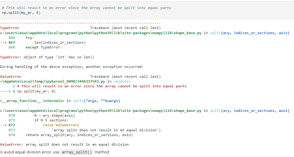
To overcome this, we can use the array_split() method.

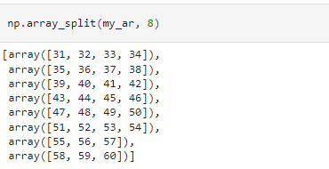
Instead of specifying the number of sub-arrays, we can pass the indices at which to split the array.

We can also use two additional methods
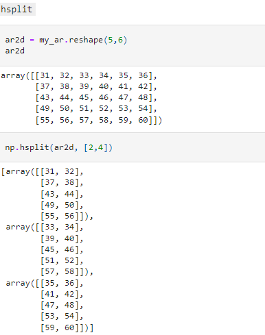
hsplit - to divide the arrays horizontally

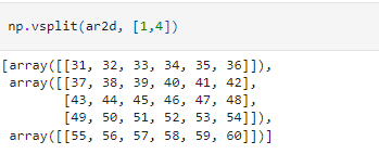
vsplit to vertically at specified indexes.

Stacking arrays.
Like the split method, we can stack (or combine) arrays. The three commonly used methods are:

Stack: as the name suggests,, this method stacks arrays. For multi-dimensional arrays, we can specify different axis along which to stack.

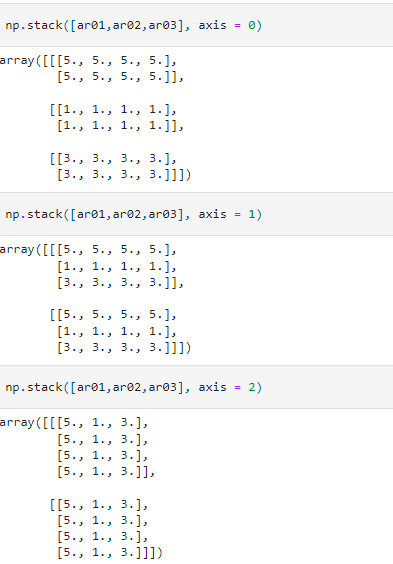
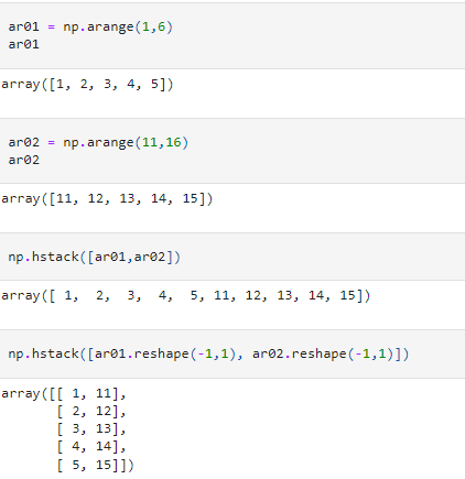
hstack: this stacks the arrays horizontally and is analogous to the hsplit() method for splitting.

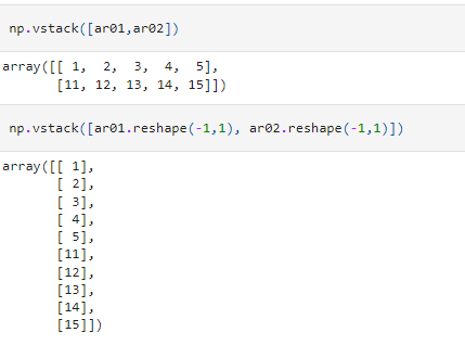
vstack: this stacks the arrays vertically and is analogous to the vsplit method for splitting.

Handling Missing Values

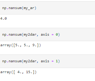
Handling missing values is a vital task in Data Science. While we want to have data without any missing values, unfortunately real-life data may contain missing values. Unlike the Pandas functions which ignore missing values automatically while aggregating, the NumPy aggregation functions do not handle missing values in a similar manner. If one or more missing values are encountered during aggregations, the resultant value will also be missing.

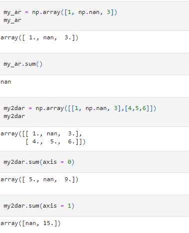
To calculate these aggregate values ignoring the missing values, we need to use the “NaN-Safe” functions. For example, the NaN-Safe version of sum – nansum() will calculate the sum of an array ignoring the missing values, nanmax() will calculate the maximum in an array ignoring the missing values, and so on.

Sorting

Another common operation encountered in Data Science is sorting. NumPy has numerous sorting methods.

The basic sort method allows sorting in ascending order.

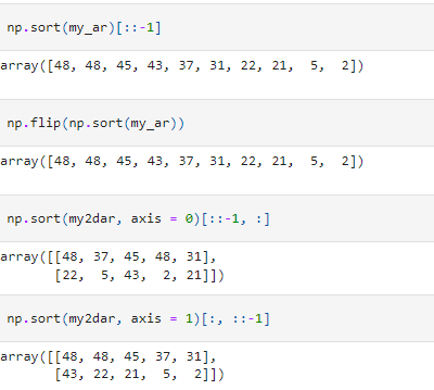
For multi-dimensional arrays, one can specify the axis to perform the sorting operation.

Note: there is no descending sort option. One can use the flip method on the sorted array to reverse the sorting process. Or use the slicer.

NumPy also has indirect sorting methods. Instead of returning the sorted array, these methods return the indexes of the sorted array. On passing these indexes to the slicer, we can get the sorted array.

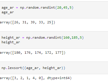
Another indirect sorting option available is the lexsort. The lexsort method allows sorting across different arrays in a specified order. Suppose there are two arrays – the first containing the age of five persons and the second containing the height. If we want to sort these on age and then height, we can use the lexsort method. The result will be the indexes that will consider both the sorting orders.

Searching

Like sorting methods, NumPy provides multiple searching methods too. The most frequently used ones are -

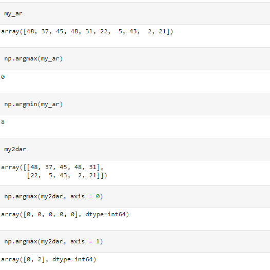
argmax (and argmin): these return the index of the maximum value (or the minimum value).

The NaN-Safe methods are also available that disregard the missing values in nanargmax and nanargmin

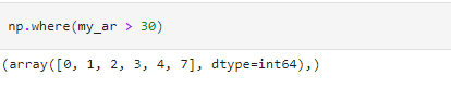
where: this returns the indexes of an array that satisfy the specified condition.

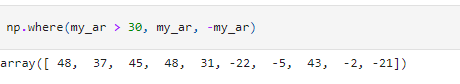
In addition, it also has the option of manipulating the output based on whether the element satisfies the condition or not. For example, if we want to return all the elements greater than 30 as positive numbers and the rest as negative numbers, we can achieve it in the following manner.

One can also perform these operations on multi-dimensional arrays.

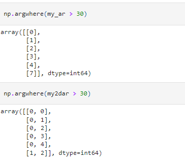
argwhere: this returns the indices of an array that satisfies where condition elementwise.

Broadcasting

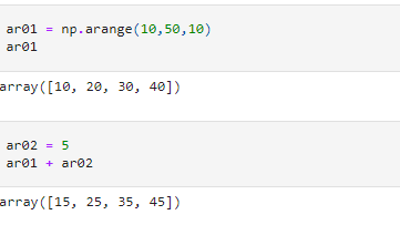
One of the most powerful concepts in NumPy is broadcasting. The broadcasting feature in NumPy allows us to perform arithmetic operations on arrays of differing shapes under certain circumstances. In the previous part of this series, we had seen how we could perform arithmetic operations on two arrays of identical shapes. Or a scalar with an array. Broadcasting extends this concept to two arrays that are not of identical shape.

However, not all arrays are compatible with broadcasting. To check if two arrays are suited to broadcasting, NumPy matches the shapes of the array element-wise, starting from the outermost axis and going all the way through to the innermost axis. The arrays are considered suitable for broadcasting if the corresponding dimensions are

• Identical
• Or at least one of them is equal to one.

To illustrate the process, let us take a few examples.

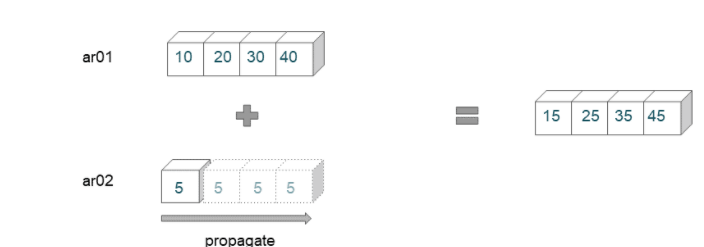
Broadcasting Example 01

Here we are trying to broadcast an array of shape (4,) with a scalar. The scalar value is propagated across the shape of the first array.

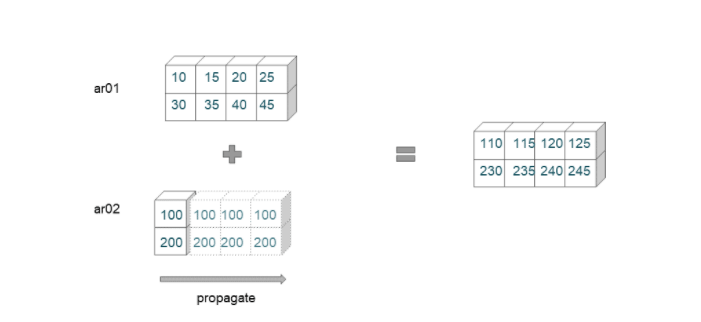
Broadcasting Example 02

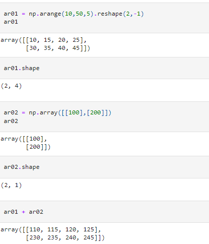
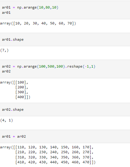
This example has two arrays of shape (2,4) and (2,1), respectively. The broadcasting rules are applied from the rightmost dimension.

• First, to match dimension 4 with dimension 1, the second array is extended.
• Then the program checks for the next dimension. Since these two dimensions are identical, no propagation is required.
• The first array and the propagated second arrays now have the same dimensions, and they can be added elementwise.

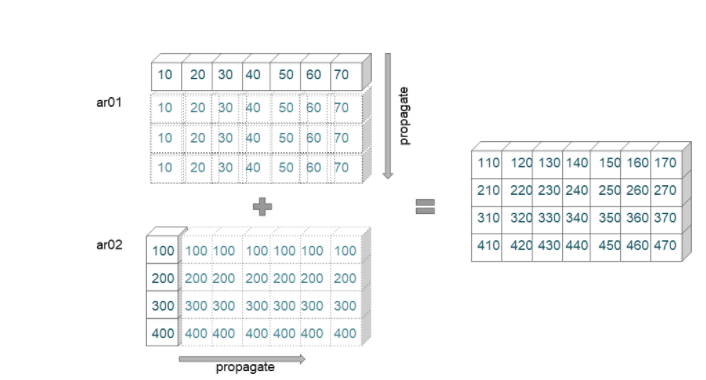
Broadcasting Example 03

In this example, we are trying to add an array of shape (7,) with an array of shape (4,1). The broadcasting proceeds in the following manner.

• We first check the rightmost dimensions (7) and (1). Since the second array dimension is 1, it is extended to fit the size of the first array (7).
• Further, the next dimensions are checked () with (4). To match the dimensions of the second array, the first array is extended to fit the size of the second array (4).
• Now the extended arrays are of dimensions (7,4) and are added elementwise.

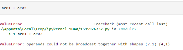
We finish off we look at two arrays that are not suited to be broadcast together.

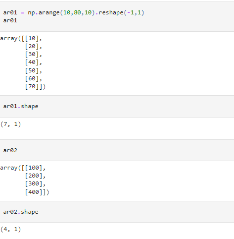
Here we are trying to add an array of shape (7,1) with an array of shape (4,1). We start with the rightmost dimension – both the arrays have 1 element each along this dimension. However, when we check the next dimensions (7) and (4), the dimensions are not compatible for broadcasting. Therefore, the program throws a ValueError.

Matrix Operations and Linear Algebra

NumPy provides numerous methods for performing matrix and linear algebra operations. We look at some of these.

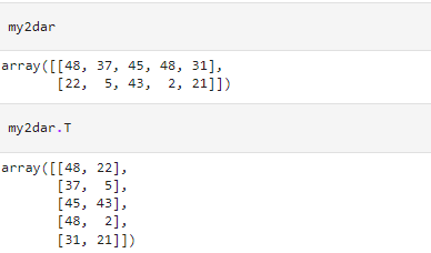
Transposing a Matrix:

For a two-dimensional array, transposing refers to interchanging rows to columns and columns to rows. One can simply invoke the .T attribute of a ndarray to get the transposed matrix.

For multi-dimensional arrays, we can use the transpose() method and specify the axis to be transposed.

Determinant of a matrix:

For square matrices, we can calculate the determinant. Determinants have numerous applications in higher mathematics and Data Science. These are used in solving a system of linear equations using the Cramer’s Rule, calculation of EigenValues which are used in Principal Component Analysis, among others. To find the determinant of a square matrix, we can invoke the det() method in the linalg sub-module of NumPy.

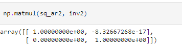
Matrix Multiplication:

Multiplying two matrices forms the basis of numerous applications in higher mathematics and Data Science. The matmul() function implements the matrix multiplication feature in NumPy. To illustrate matrix multiplication, we multiply a matrix with the identity matrix created using the eye() method. We should get the original matrix as the resultant product.

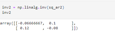
Inverse of a matrix:

For a square matrix M, the inverse of a matrix M-1 is defined as a matrix such that M M-1 = In where In denotes the n-by-n identity matrix. We can find the inverse of a matrix in NumPy by using the inv() method of the linalg submodule in NumPy.

We can verify that product of a matrix and its inverse equals the identity matrix.

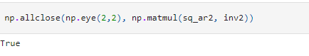
Equality of NumPy arrays.

Given the differences in floating-point precision, we can compare if two NumPy arrays are element-wise equal within a given tolerance. This can be done using the allclose method.

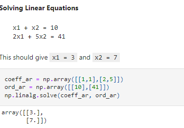
Solver.

The linalg module of NumPy has the solve method that can compute the exact solution for a system of linear equations.

Polynomials

Like the linear algebra sub-module, NumPy also supports polynomials algebra. The module has several methods as well as the Polynomial class that contains the usual arithmetic operations. Let us look at some functionalities of the polynomial sub-module. To illustrate this, we use the polynomial in x f(x) as

f(x) = x² - x - 6

we can create the polynomial from the coefficients. Note, coefficients must be listed in increasing order of the degree. So the coefficient of the constant term (-6) is listed first, then the coefficient of x (-1), and finally the coefficient of x² (1)

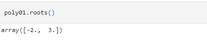
The expression can also be factorized as

f(x) = (x-3)(x+2)

Here 3 and -2 are the roots of equation f(x) = 0. We can find the roots of a polynomial by invoking the roots() method.

We can form the equation from the roots using the fromroots() method.

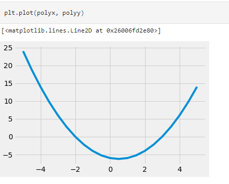
The polynomial module also contains the linspace() method that can be used to create equally spaced pairs of x and f(x) across the domain. This can be used to plot the graph conveniently.

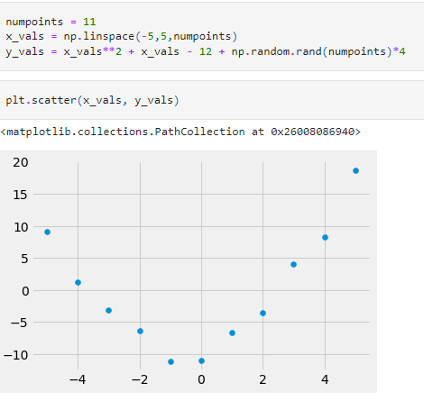
Curve Fitting

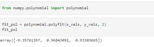
NumPy polynomial sub-module also provides the least-squares fit of a polynomial to data. To illustrate this, let us create a set of data points and add some randomness to a polynomial expression.

We then invoke the polyfit() method on these points and find the coefficients of the fitted polynomial.

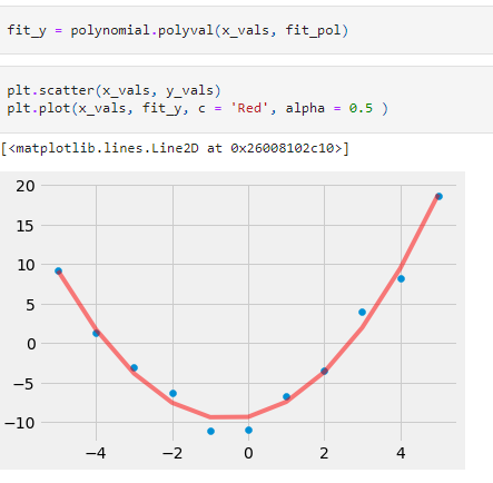
We can also visually verify the fit by plotting the values. To do this we use the polyval method to evaluate the polynomial function at these points.

Importing and Exporting Data in NumPy

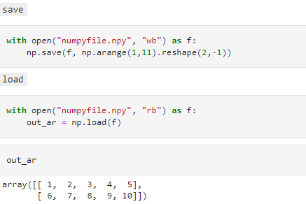
Till now we have created arrays on the fly. In real-life Data Science scenarios, we usually have the data available to us. NumPy supports importing data from a file and exporting NumPy arrays to an external file. We can either use the save and load methods to export and import data in native NumPy native (.npy and .npz formats).

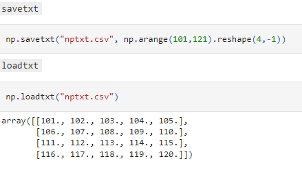
We can also read from and write data to text files using the loadtxt and savetxt methods.

Conclusion

In this series, we looked at NumPy which is the fundamental library in the Python Data Science ecosystem for scientific computing. If you are familiar with Pandas, then moving to NumPy is very easy. Comfort with NumPy is expected from an aspiring Data Scientist or Data Analyst proclaiming proficiency in Python.

As with any skill, all one needs to master NumPy is patience, persistence, and practice. You try these and many other data science interview questions from actual data science interviews on StrataScratch. Join a community of over 40,000 like-minded data science aspirants. You can practice over 1,000 coding and non-coding problems of various difficulty levels. Join StaraScratch today and make your dream of working at top tech companies like Apple, Netflix, Microsoft, or hottest start-ups like Noom, Doordash, et al a reality. All the code examples are available on Github here.