Machine Learning in R for Beginners: Super Simple Way to Start

Beginner's Guide to Machine Learning with R: Learn to install RStudio, handle data, and build models like linear regression and neural networks.

"R or Python? Which should you choose for data science and machine learning? Most people who work in these fields want to know the answer to this question.

Even if you choose Python, give R a chance. Let’s explore how R, with its powerful packages and IDEs, provides an excellent environment for machine learning, especially for beginners.

We’ll start with the basics and apply deep learning to dive deep into the ocean. So, let’s get started!

Getting Started with R

Before going into the Machine Learning with R, let’s first install RStudio.

You can download it from the CRAN (Comprehensive R Archive Network) there.

After installing R, you can download RStudio, IDE for R, which simplifies coding and includes various tools to help you visualize your data and output.

RStudio can be downloaded from here.

Basic R Syntax and Operations

R has unique syntax and operations. Let’s see a short overview.

• Variables and assignment: Use <- or = to assign values, - x <- 5
• Functions: Call functions using parentheses - sum(x, y)
• Data structures: Include vectors, lists, data frames, and matrices.
• Indexing: Access elements in data structures with brackets - vector[1] or dataframe$column.

Getting comfortable with these basics will give you a great start. These will help you read this one if you are a total stranger.

Model Building on a Synthetic Dataset

We'll use this data project to show how to apply machine learning in R. You can find details from this project on our platform here, where we solved it using Python. Here is the assignment:

Here is the data description.

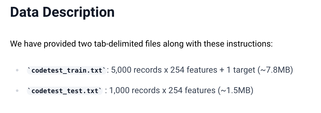
Loading Your Data

To begin your machine learning project, you must first load your data. It involves specifying the location of your data files and using R to import them to analyze them.

# Set the file paths
train_file <- "path of the file on your PC."
test_file <- "path of the file on your PC."

# Import data into R
train_data <- read.table(train_file, header = TRUE, sep = "\t")
test_data <- read.table(test_file, header = TRUE, sep = "\t")

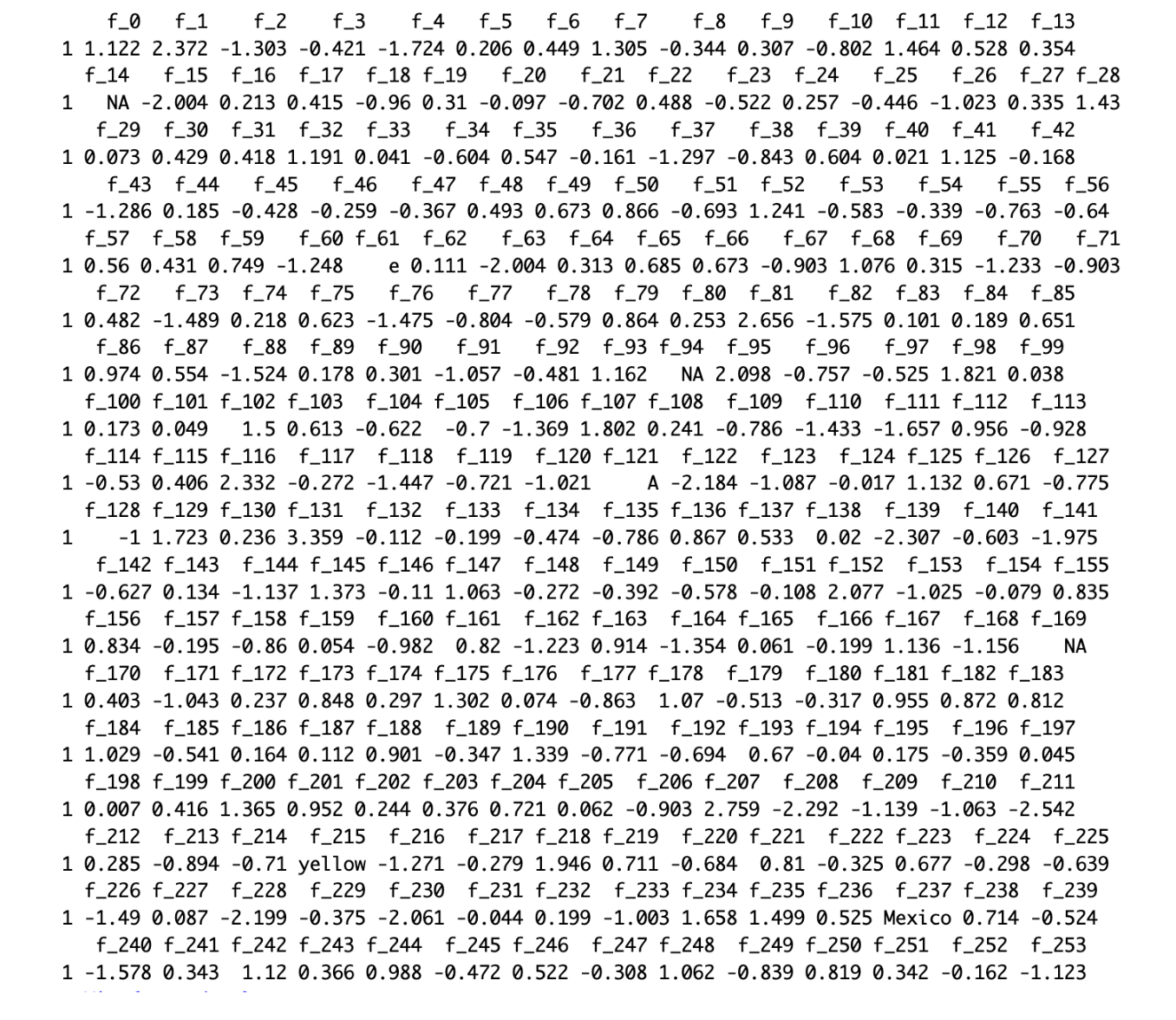
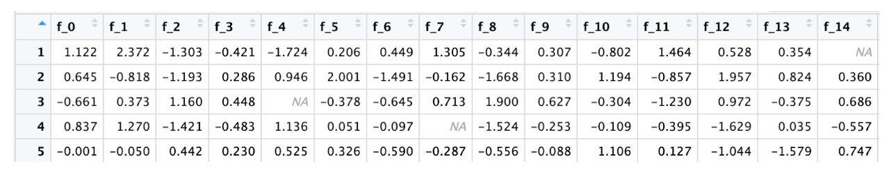
head(train_data,1 )

The code above sets the file paths to your training and testing datasets and imports them using read.table, a function suited for reading tab-separated values. head(train_data,1) displays the first entry of your training dataset, helping you verify that data is loaded correctly.

Here is the output:

You can also repeat the same code for test data or simply click on the dataset name in the upper right corner, under environment, on R studio.

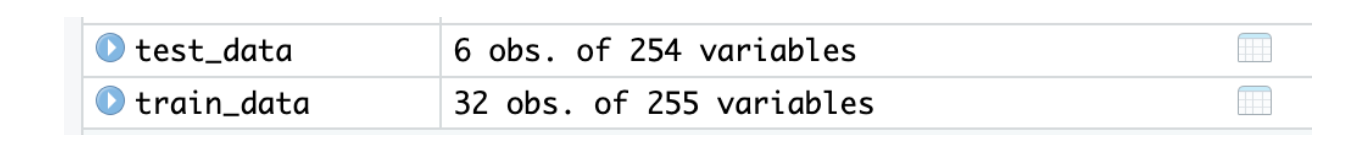
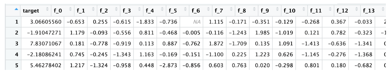
And you can see your data in a more structured way. Here is the train data

Here is the test data

Missing Value Detection

Identifying missing values in your dataset is crucial before any analysis. Missing data can influence your analysis's outcome, so it must be handled appropriately.

As you can see, our data contains NAs. We need to remove them before starting the analysis.

# Check for missing values in the training dataset
missing_train <- sum(is.na(train_data))

# Check for missing values in the test dataset
missing_test <- sum(is.na(test_data))

# Print the number of missing values in each dataset
cat("Number of missing values in the training dataset:", missing_train, "\n")

This step would involve using functions like is.na() to detect missing values across your dataset and summarizing them to understand the extent of missingness.

Here is the output:

Let’s see the test set.

cat("Number of missing values in the test dataset:", missing_test, "\n")

Now it is time to remove those NA’s.

train_data <- na.omit(train_data)
test_data <- na.omit(test_data)

We remove Na’s. Now, let’s find out if we did successfully.

# Check for missing values in the training dataset
missing_train <- sum(is.na(train_data))

# Check for missing values in the test dataset
missing_test <- sum(is.na(test_data))

cat("Number of missing values in the training dataset:", missing_train, "\n")

Here is the output;

Let’s see the test set.

Great, now our dataset is clean.

Data Normalization

Data normalization is an essential preprocessing step in machine learning. Normalization ensures that all features of the dataset have the same scale. This is important because many machine learning models perform well when the features are on a similar scale, as significant differences in magnitude give certain features more dominance over others.

We will normalize the datasets in our implementation using the R’s scale() function. The scale () function standardizes each dataset column with a mean of 0 and standard deviations 1. By standardizing all the features to a standard scale, we allow the machine learning model to learn from the data without the dominance of some features.

Here is the code:

# Convert non-numeric columns to numeric in the training dataset
train_data_numeric <- sapply(train_data, as.numeric, na.rm = TRUE)

# Convert non-numeric columns to numeric in the test dataset
test_data_numeric <- sapply(test_data, as.numeric, na.rm = TRUE)

# Perform data normalization on the numeric training dataset
normalized_train <- scale(train_data_numeric[, -ncol(train_data_numeric)])

# Perform data normalization on the numeric test dataset
normalized_test <- scale(test_data_numeric)

# Check the first few rows of the normalized training dataset
head(normalized_train)

Here is the output.

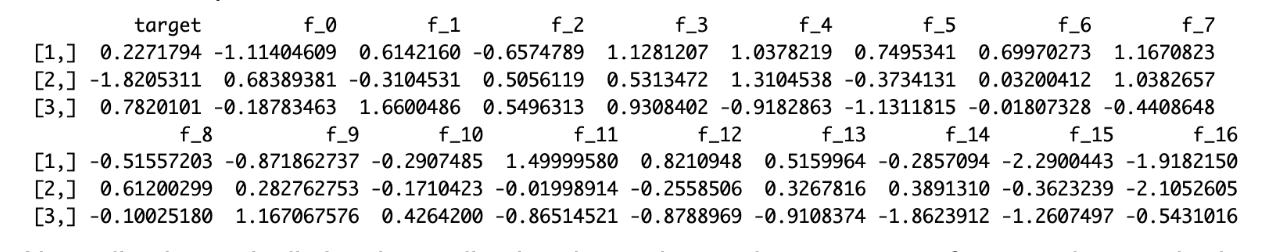
Normalization typically involves adjusting data values to have a mean of zero and a standard deviation of one. It is usually done using the scale() function in R. Now, let’s see the test set.

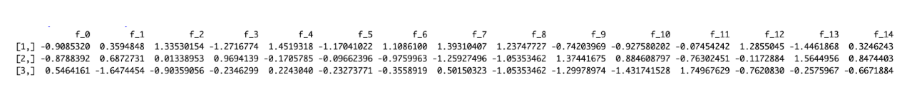
# Check the first few rows of the normalized training dataset
head(normalized_test)

Here is the output.

Splitting Data into Training and Test Sets

You should split your dataset into train and test subsets until you can feed your machine-learning model with data. The main idea of the scheme laid down in the previous sentence is to understand how good your models are in predicting a response based on a new matrix of observations. In other words, we will determine their generalization ability.

Our data was already split, so we don't need to split it into training and test sets, but for the sake of this one, let’s split our training data into the training and test sets.

Now, let’s do this. Here is the code.

# For repeatability, set the seed.
set.seed(123)

# Give the proportion of data to be used for testing.
test_size <- 0.2

# Calculate the number of rows for the test set
test_rows <- round(nrow(train_data) * test_size)

# Get the test set's row count
test_indices <- sample(seq_len(nrow(train_data)), size = test_rows)

# Create the training and test sets
training_set <- train_data[-test_indices, ]
test_set <- train_data[test_indices, ]

# Check the dim of the training and test sets
cat("Training set size:", nrow(training_set), "\n")

It involves using functions like createDataPartition() from the caret package, ensuring a reliable division for training and evaluating your model. Let’s see the output:

Here is the code to find the test set size:

cat("Test set size:", nrow(test_set), "\n")

Here is the output;

Data Preparation

Preparing the data before building machine learning models is crucial. In machine learning, you must ensure that all your features are in numerical format.

This section will first explore the steps to prepare our Data for Machine Learning in R. Let’s start!

Identifying Non-Numeric Columns

First, we'll identify columns with non-numeric data types in the training and test datasets.

# Let’s find out columns have non-numeric data types.
non_numeric_cols <- names(train_data)[sapply(train_data, function(x) !is.numeric(x))]

# Print these columns- non numeric
if (length(non_numeric_cols) > 0) {
  cat("Columns with non-numeric data types:", non_numeric_cols, "\n")
} else {
  cat("All columns have numeric data types.\n")
}

Here is the output.

# Identifying non-numeric columns in the test dataset
non_numeric_cols_test <- names(test_data)[sapply(test_data, function(x) !is.numeric(x))]

# Print columns with non-numeric data types in the test dataset
if (length(non_numeric_cols_test) > 0) {
  cat("Columns with non-numeric data types in the test dataset:", non_numeric_cols_test, "\n")
} else {
  cat("All columns in the test dataset have numeric data types.\n")
}

Here is the output.

Encoding

Encoding is the process of changing your non-numerical features into numerical ones. As we said before, you need to encode to apply a machine learning model because your model understands and learns just from numbers.

Here, we use simple encoding techniques to convert categories into numeric identifiers. Here is the code.

library(data.table)  
library(mlr3misc)    

for (feature in non_numeric_cols) {
  train_data[[feature]] <- as.integer(factor(train_data[[feature]]))
}

# Encoding non-numeric features in the test dataset
for (feature in non_numeric_cols_test) {
  test_data[[feature]] <- as.integer(factor(test_data[[feature]]))
}

We've changed all text data in both datasets into numbers with this code. Next, we’ll verify it.

Verification of Encoding

Once the non-numeric features are encoded into numeric values, you must verify. This can be done by examining the features’ data types and unique values within the encoded features.

# Checking the data types in the training set
cat("Data types of features in the training dataset:\n")
print(sapply(train_data, class))

# Check the data types in the test set
cat("\nData types of features in the test dataset:\n")
print(sapply(test_data, class))

# Check the unique values of encoded features in the training dataset
cat("\nUnique values of encoded features in the training dataset:\n")
print(sapply(train_data[non_numeric_cols], unique))

# Check the unique values of encoded features in the test dataset
cat("\nUnique values of encoded features in the test dataset:\n")
print(sapply(test_data[non_numeric_cols_test], unique))

Here is the output.

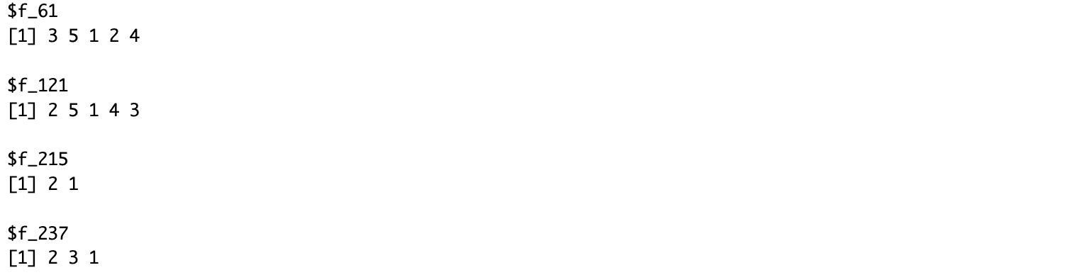
The non-numeric features have been encoded into numeric values. Furthermore, each feature has a unique integer representation. Therefore, the entire encoding process was successful.

This means that the data has been prepared appropriately and is ready for the subsequent processes in the machine-learning workflow.

Building Linear Regression Model

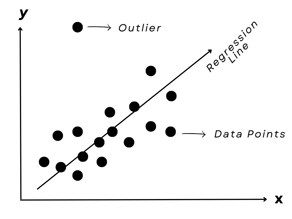
Now, let’s start with a simple algorithm: linear regression. Linear regression is a basic predictive model that assumes a linear relationship between the input variables (X) and the single output variable (Y).

Here is the code to do that.

# Assuming 'target' is the column name for your dependent variable in your datasets
# Separating features and target variables from the normalized training data
y_train <- training_set[["target"]]
X_train <- training_set[, setdiff(names(training_set), "target")]

# Separating features and target variables from the normalized test data
y_test <- test_set[["target"]]
X_test <- test_set[, setdiff(names(test_set), "target")]

# Fitting the linear regression model using the training data
lm_model <- lm(y_train ~ ., data = as.data.frame(X_train))

# Summarizing the model to get insights into coefficients and statistics
summary(lm_model)

# Making predictions on the test data
predictions <- predict(lm_model, newdata = as.data.frame(X_test))

# Calculating the Mean Squared Error (MSE) for the test data
mse <- mean((predictions - y_test) ^ 2)

# Printing the MSE to understand the average squared difference between the estimated values and actual value
print(paste("Mean Squared Error on Test Set:", mse))

Here is the output.

If you are confident about your Machine Learning model and thrive on showing it to the world, you need to know more about Machine Learning Operations. Check this one out to learn more.

Decision Tree

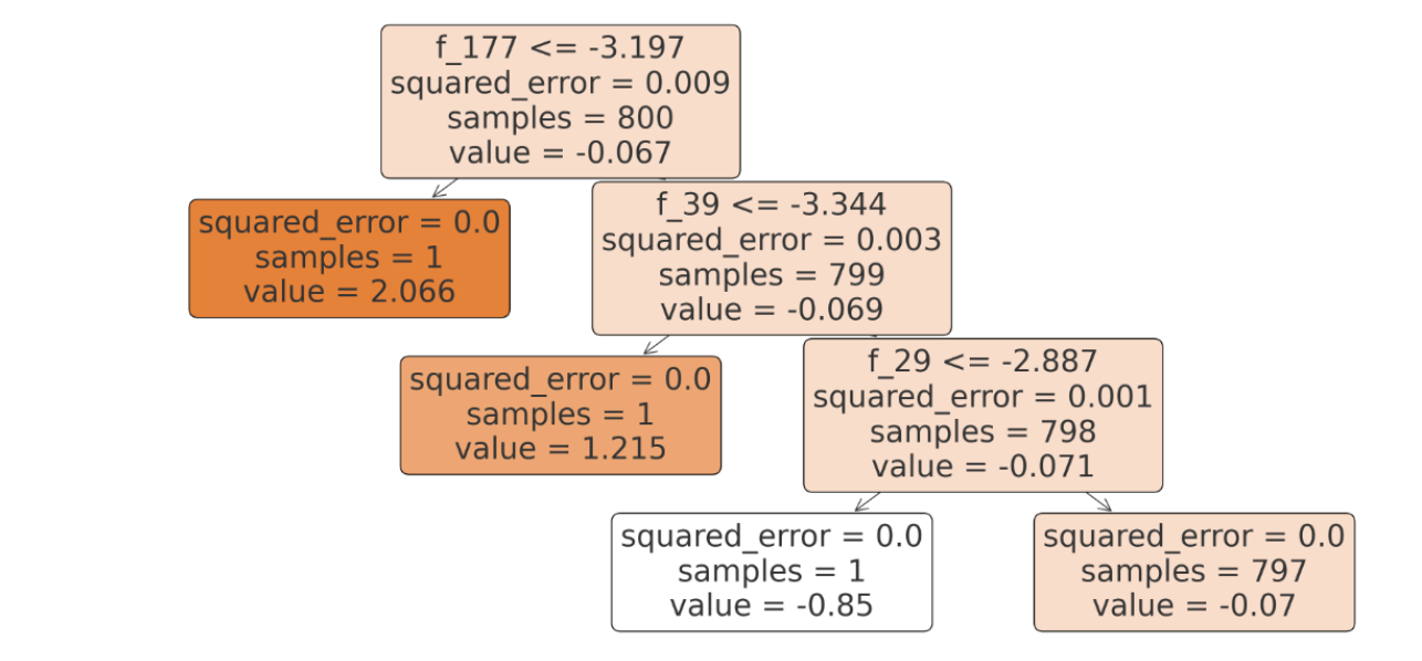
Decision trees are the go-to algorithm for performing both classification and regression tasks. They divide the dataset into branches to form a tree for decision-making. In this example, we’ll use a decision tree for regression.

Here is the code.

library(tree)

# Build the regression tree model
tree_model <- tree(formula = target ~ ., data = training_set)

# Display information about the tree
summary(tree_model)

# Plot the tree
plot(tree_model)
text(tree_model, pretty = 0)

# Predict using the regression tree
predictions_tree <- predict(tree_model, newdata = test_set)

# Optional: Evaluate the performance of the model with Mean Squared Error
y_test <- test_set$target  # Assuming 'target' is the actual response variable in your test set
mse <- mean((predictions_tree - y_test)^2)

# Print the Mean Squared Error
print(paste("Mean Squared Error:", mse))

Here is the output.

As you can see, the MSE error decreases because we are using a more complex algorithm.

Support Vector Machines

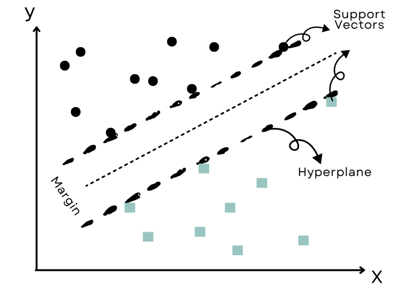
Support Vector Machines (SVM) are powerful classification models that work well on linear and non-linear data. Here is the code.

library(e1071)

# Assuming 'target' is your response variable and the data is split into training_set and test_set
svm_model <- svm(target ~ ., data = training_set, kernel = "radial", cost = 10, scale = TRUE)
summary(svm_model)

You train an SVM model using the svm() function from the e1071 package. The function parameters can be adjusted to improve the model's accuracy. Here is the output:

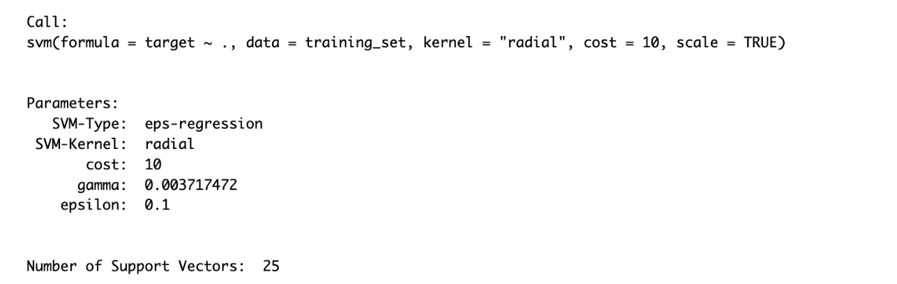
Let’s evaluate this output because it differs slightly from other algorithms.

• SVM-Type: eps-regression - Optimized for predicting continuous outcomes with an error threshold.
• SVM-Kernel: radial - Uses RBF kernel to handle non-linear data effectively.
• Cost: 10 - Balances between fitting data well and avoiding overfitting.
• Gamma: 0.00371472 - Low gamma, indicating broad, smooth decision boundaries.
• Epsilon: 0.1 - Allows minor prediction errors without penalty, enhancing model robustness.
• Number of Support Vectors: 25 - Shows an efficient and potentially well-generalized model.

To learn more about Machine Learning Algorithms, visit this one.

Neural Networks

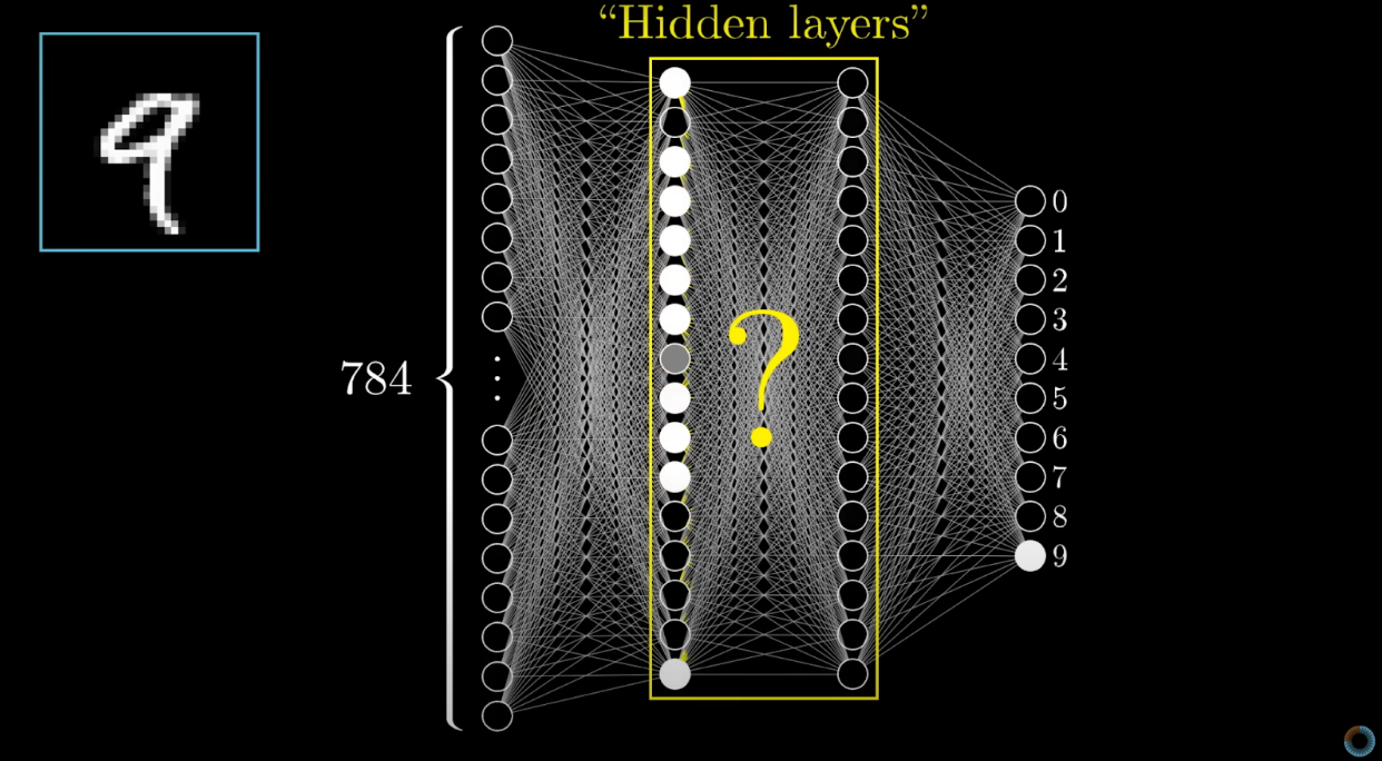
Neural networks are a class of models in the general machine-learning literature designed to imitate the interconnected neuron structure of the human brain.

They excel at mathematically defining non-linear relationships in data. For example, smaller neural networks can be built with the nnet package in R, while more complicated networks requiring deep learning can be built using the Keras package.

library(nnet)

# Training a simple neural network model
nn_model <- nnet(target ~ ., data = training_set, size = 3, linout = TRUE)
summary(nn_model)

# Prediction
nn_predictions <- predict(nn_model, newdata = test_set, type = "raw")
mse_nn <- mean((nn_predictions - test_set$target)^2)
print(paste("MSE:", mse_nn))

You would use the nnet() function from the nnet package to train a neural network. This process includes visualizing the network's performance and adjusting parameters like the number of neurons. Here is the output.

If you want to learn neural networks from scratch, you can watch this YouTube series from 3Blue1Brown. It is straightforward and beginner-friendly.

Conclusion

As you can see from the results, the results improve when the algorithms you use get more complex. In this one, you’ll discover machine learning in R, starting with fundamental concepts like installing R and going deep into the rabbit hole by applying deep learning.

After learning, it is time to use your skills in real-life challenges, like data projects from different companies and interview questions. You can see these examples here on our platform. See you there!