How to Create Pivots in SQL (with examples)

Categories:
 Written by:
Shivani Arun
Reshaping data using Pivots is table-stakes in data science. Learn about its importance, techniques, and implementation.
Pivoting data in SQL is an approach used daily by data scientists to reshape data from rows to columns. This article covers three commonly used approaches to pivot data in SQL, starting using the native PIVOT() to leveraging CROSSTAB and then finally moving on to more dialect-agnostic approaches (e.g., CASE WHEN with Aggregation).
Moving beyond Excel pivot tables allows you to scale using SQL and effectively access and analyze petabytes of data.
What Does “Pivot in SQL” Mean?
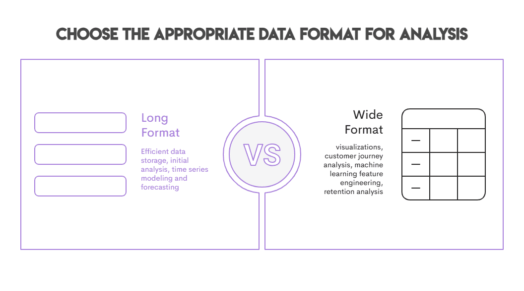
Data is rarely in the shape or form you need for analysis. Pivoting transforms data from its commonly stored long format (stacked rows) to wide format (columns), making it easier to compare, visualize, and derive insights. For those of us who have created pivot tables in Microsoft Excel, pivoting in SQL works by reshaping rows to columns for data analysis, reporting, and in many more use cases.
Let’s take the example of a simple dataset representing sales data for a company. The data includes information about the region, product category, and sales amount.
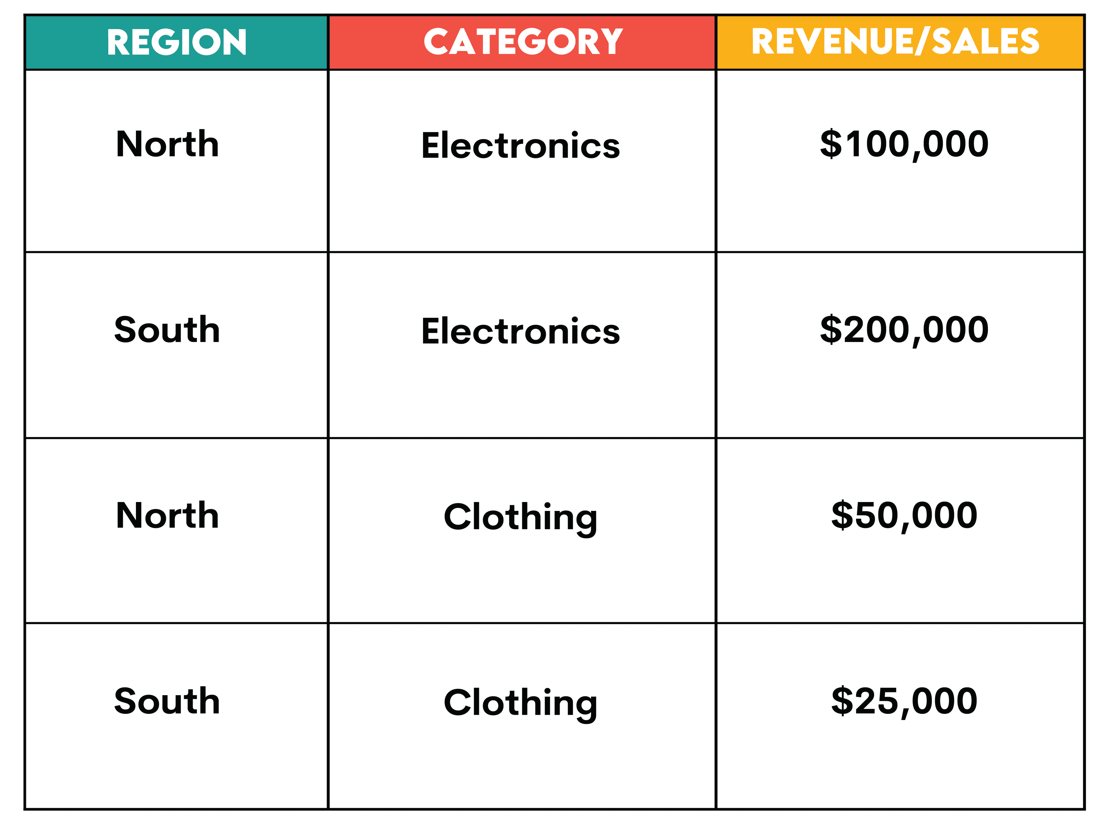
1. Original Data (Long Format/Rows)
Each row represents one transaction. This format can be modified by adding new rows without altering the format of the table, and storing data in long format is generally more efficient. As you practice SQL interview questions, notice that most tables that reference entities such as transactions, orders, and customers are all represented in long format with one row for unique keys such as transaction_id, order_id, customer_id.
2. Pivot Table Format
We can create a pivot table to reshape this data where "Region" is the row index, "Category" is the column index, and "Sales/Revenue" is the value.
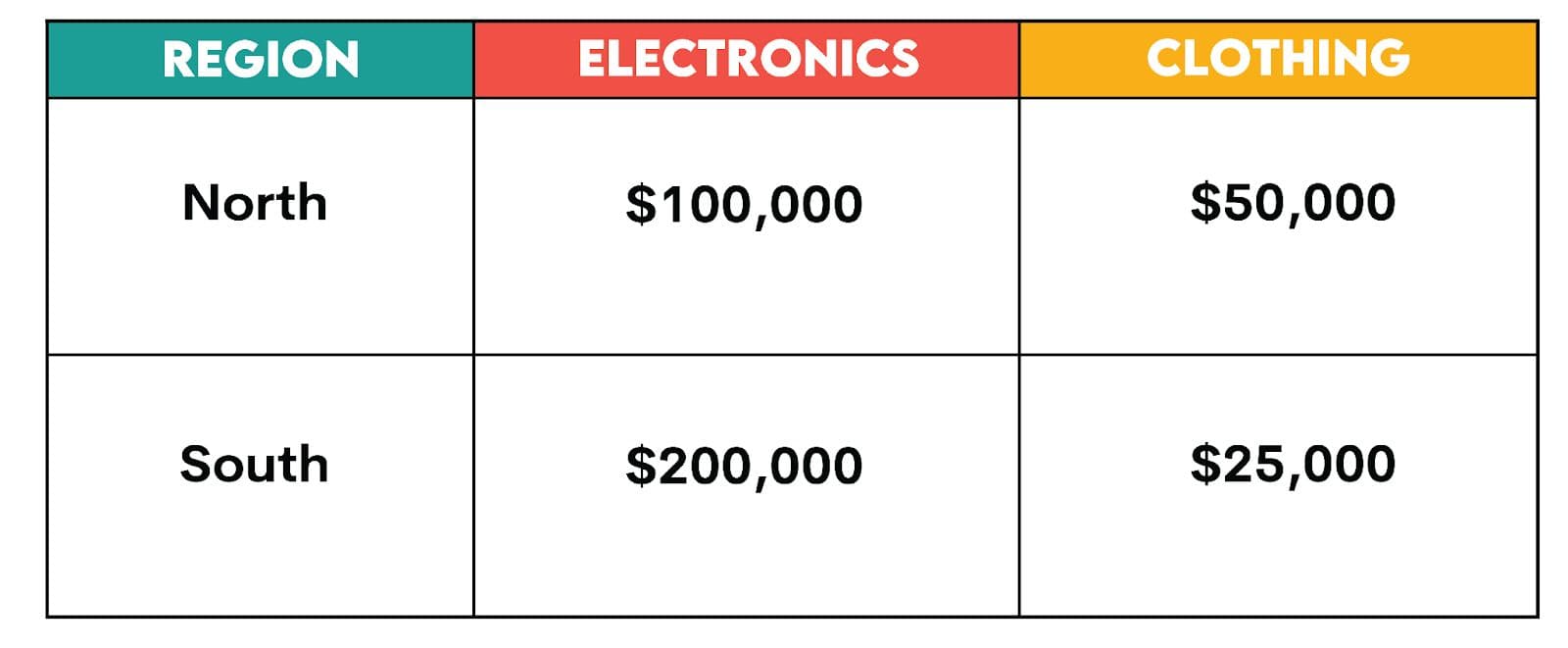
3. Reshaped Data (Wide Format/Columns)
The pivot table then restructures the data, creating a new table where:
- Rows: Represent the unique values from the "Region" column (North, South).
- Columns: Represent the unique values from the "Category" column (Electronics, Clothing)
- Values: Represent the aggregated "Sales" amounts, calculated for each combination of Region and Category.
The newly pivoted data will now look like:
When and Why Do We “Pivot”?
Intuitively, we can see the value of pivoting from the previous example, as it makes reporting quite clear and understandable. In the day-to-day of a data scientist, one of the most critical skills is simplifying the analysis to explain it to non-technical audiences who have the latitude to make decisions based on this data. Pivoting data to display it side-by-side (in columns) in reports and visualizations is a crucial approach.
Most importantly, having an intuition of what ‘gold’ is hidden in the data is easier if you zoom into these side-by-side comparisons and understand the trends and patterns, especially when comparing categorical data (E.g., ‘Electronics’ vs ‘Clothing’ categories).
Now let’s look at use cases that define the value of using pivots on the job:
Common Use Cases for Pivoting:
1. Machine Learning Feature Engineering: Many machine learning algorithms use data where user or time period is a row and features are given in columns. It also makes sense to create ratios, percentages, and features that represent how different variables interact with each other. Moreover, most categorical variables can be represented as separate features in a wide format. Let’s take a look at two examples:
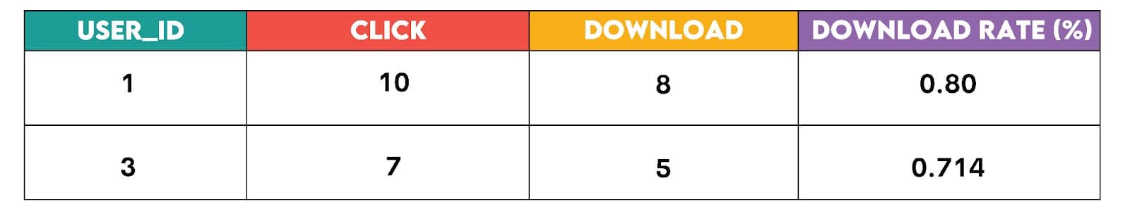
Intuitive Feature Creation: Reshaping data from long to wide format can be used to create ratios, percentages, and interaction features (representing the combined effect of two or more features) as columns. For example, let’s look at a table with user interactions. One of the features that you want to engineer is the download rate (%) for each user, given by download/click.
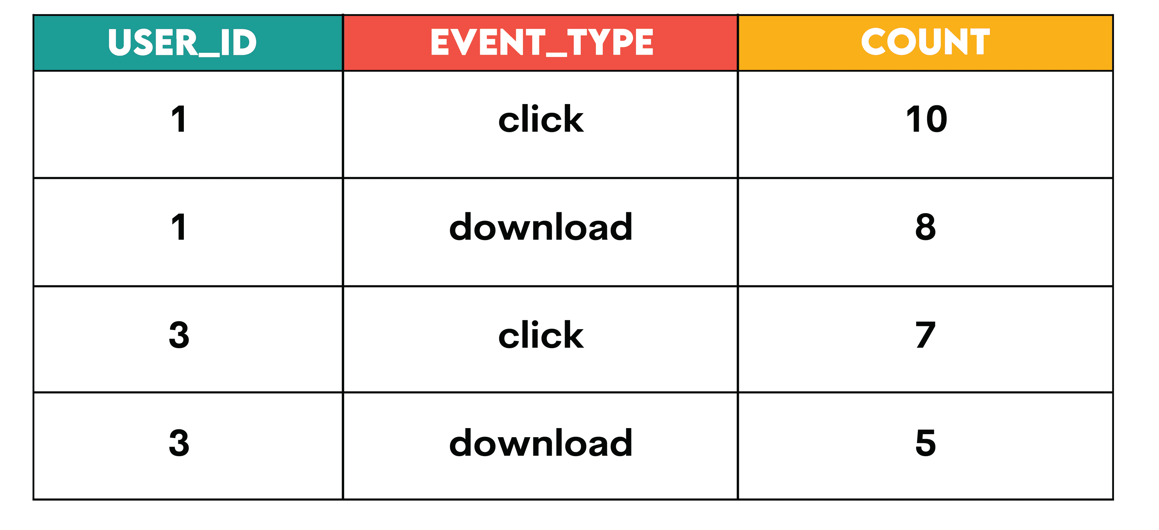
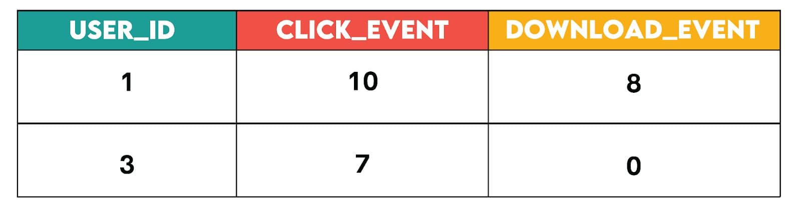
Using pivoting, we can reshape this data into a wide format:
A multitude of features that feed into several types of machine learning/prediction models are based on this approach.
Let’s look at another example: Have you heard of one-hot feature encoding? It’s a fancy name for pivoting data that represents categories (categorical data) from long format to wide format.
Categorical variables can be each represented in their own columns using pivoting. This is used in data science algorithms that cannot directly handle categorical data. For example, this table below shows this in practice:
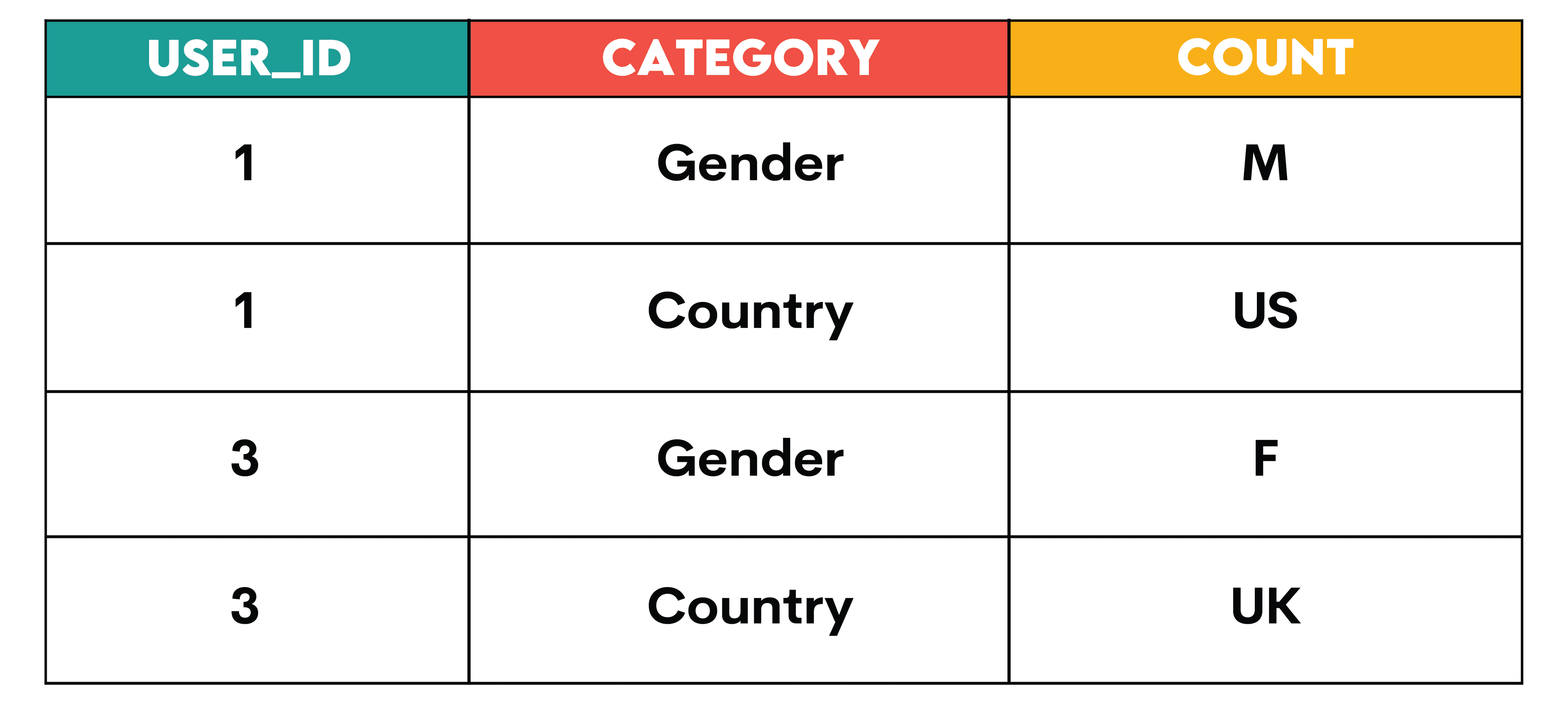
Here’s how the algorithm would be given the data:
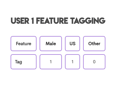
‘1’ simply represents a Yes and ‘0’ a No in the above data.
2. User Retention Analysis
Cohort analysis, which tracks users across time to understand churn and retention patterns, relies on no surprises in pivoting for intuitive visualizations. By pivoting the data, we can easily see how many users from each cohort are retained over time. This theme is also a favorite theme that appears in advanced SQL interview questions, so be sure to prepare for it.
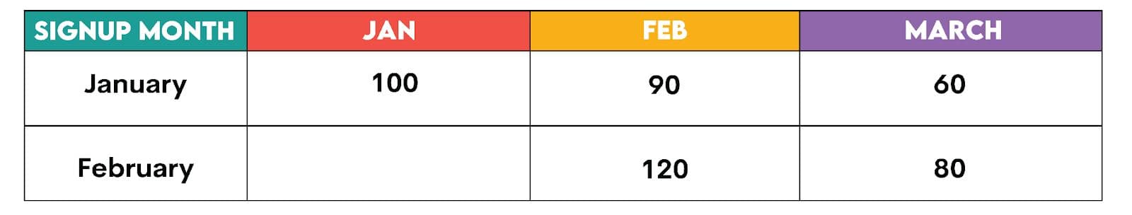
As an example, the above pivoted data allows us to easily compare the retention rates of different cohorts. For example, we can see that 80% of the January cohort was retained in February, while 75% of the February cohort was retained in March.
3. Customer Journey Analysis
Funnel analysis comparing different user segments is yet another commonplace example. Below is a sample table that displays funnel steps as columns and segments as rows:
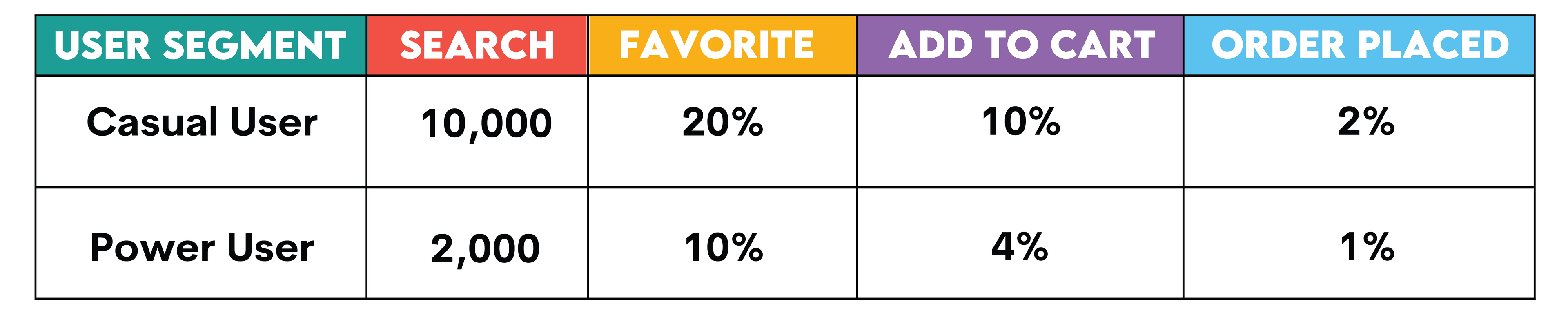
The value of data insights depends on how effectively they can be communicated and acted upon—pivoting is essential for achieving this goal. There are many ways that you can now visualize this data. Here’s a simple but powerful visual for our power users:
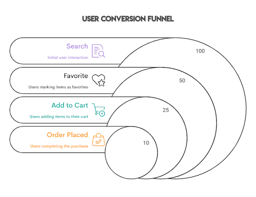
- Search: The initial point where users begin their interaction.
- Favorite: Users marking items as favorites, indicating interest.
- Add to Cart: Users adding items to their cart, showing purchase intent.
- Order Placed: Users completing the purchase process.
Before we dive into building this foundational skill in SQL, let’s understand when to use SQL compared to other languages, e.g., Python.
Why Use SQL for Pivoting Instead of Python?
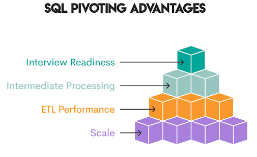
While Python libraries like Pandas offer powerful data reshaping capabilities (e.g., stack, unstack, pivot_table, melt), SQL offers distinct advantages:
- Scale: SQL handles massive datasets that cannot be loaded into memory
- ETL Performance: Pivots leverage database indexing and optimization
- Intermediate Processing: Create reshaped tables before final analysis
- Interview Readiness: Pivoting is a common technical interview topic
Pro Tip: Push heavy filtering and critical pivots to SQL to shrink large datasets, then pull summarized results into Python for flexible final analysis (e.g., w/ Pandas)
Before we jump into how to pivot, another question that may be top of mind is what is the difference between standard GROUP BY and aggregation and pivot, and the scenarios where each of them is used in the day-to-day life of a data scientist.
Difference between GROUP BY / Aggregation and Pivoting
Very simply, PIVOT is GROUP BY + Data Transformation!
GROUP BYcollapses rows based on grouping columns and applies aggregate functions (SUM(),COUNT(),AVG(), and so on). The result stays in a vertical/long format unless we explicitly reshape the data.- Pivoting takes values from rows and transforms them into columns. It rotates the data from a vertical to a horizontal layout. This means that pivoting involves the use of
GROUP BYand then reshapes the data from vertical/long format to wide format (e.g., throughCASEstatements)
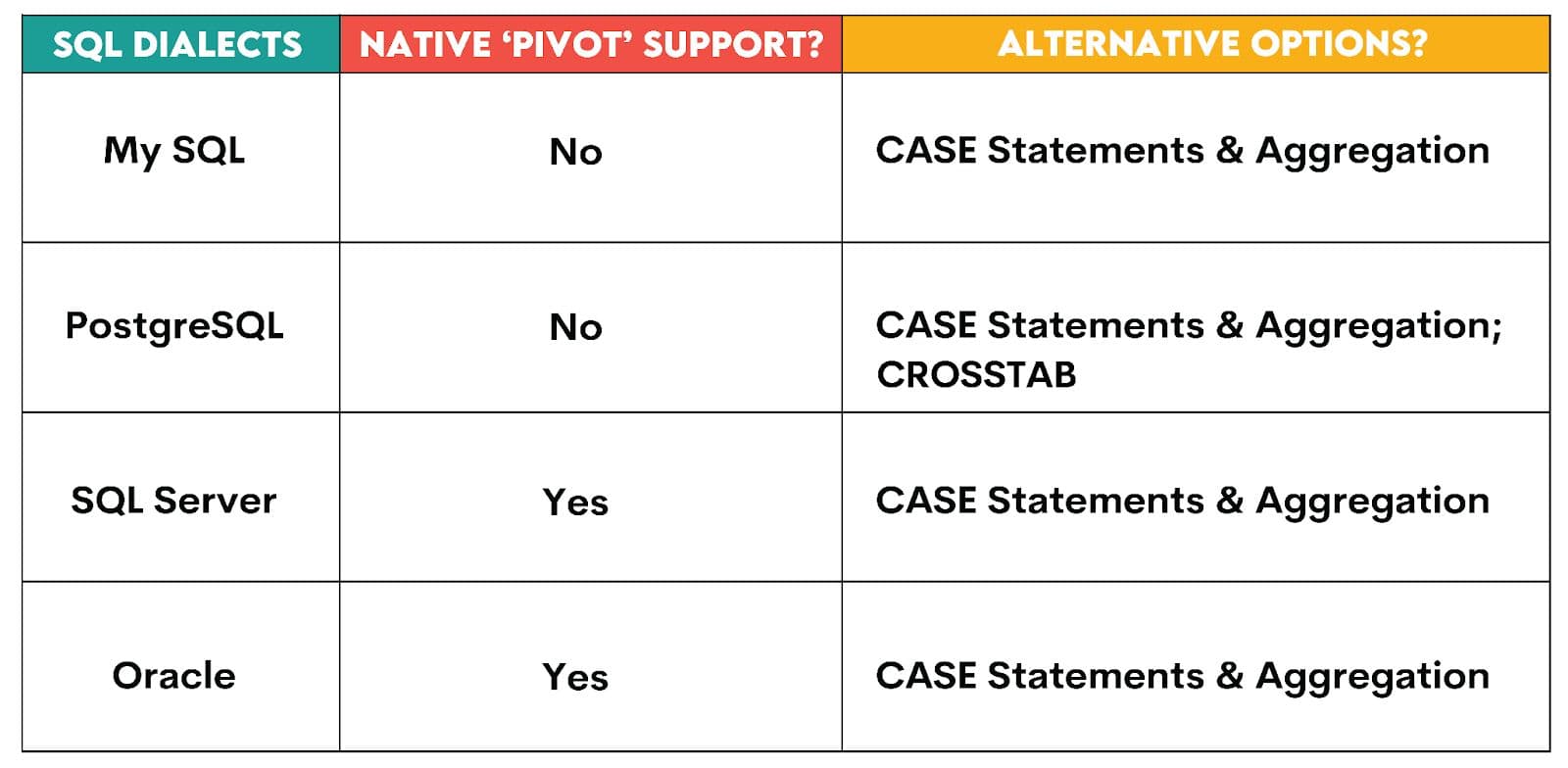
With this solid foundation on PIVOTING, let’s jump into understanding which SQL dialects can be leveraged to implement a native PIVOT().
SQL Dialects & Support (Which SQL Engines Support Native PIVOT?)
Basic Static Pivot: The PIVOT Syntax in SQL Server / Oracle
To understand the approach to general PIVOT syntax, let’s first understand the three steps involved:
- Prepare source data: Select columns of interest (month, service_name, monetary_value)
- Aggregate Functions & PIVOT: Write the aggregate function and which column values become new columns
- Select final output: Choose which pivoted columns to display
Now let’s apply this syntax to one of the questions in the StrataScratch platform:
Total Monetary Value Per Month/Service
Last Updated: June 2021
Find the total monetary value for completed orders by service type for every month. Output your result as a pivot table where there is a column for month and columns for each service type.
Our goal in this question is to find the total monetary value for completed orders by service type for every month. The output is a pivot table with a column for month and columns for each service type.
Here’s a link to the question: https://platform.stratascratch.com/coding/2047-total-monatery-value-per-monthservice
Tables:
Before diving into the solution, break this problem into steps to understand how to pivot the data. There are 3 main steps in the approach:
- Filter for completed orders only (prepare source data)
- Group by month and aggregate monetary values by service type (aggregate function & pivot). Return the final results in wide format, with each service type as its own column
- Select the final output and choose which columns to display (select final output)
Solution: To transform service types from rows into columns, we need to pivot the service_name column from long format to wide format.
To summarize, let's break down the PIVOT:
- Source subquery: Filters and selects month, service_name, and monetary_value
- Grouping column: month
- Aggregate function: SUM()
- Pivot column: service_name (values become column names)
- Value column: monetary_value
- IN clause: Lists all service types to create as columns
Once you get used to it, you will observe that the PIVOT function has a very readable syntax. Readable code is a boon when you are reviewing exercises that you did a few months ago!
Handling NULLs / Missing Data / Default Values
Let’s first discuss how to handle NULLs and default values.
1. Handling NULLs & Default Values
While reshaping the data or while doing any analysis, understanding the presence of null values and replacing them is critical to ensure that the final report is formatted for end-user consumption or further analysis and visualization.
Similarly, if you are building a machine learning model, null values have to be treated in various ways depending on conditions, such as whether the value was missing at random or if the values were intended to be 0 instead.
Ever tried creating a graph when columns have NULL values? You will end up getting errors and will not be able to render most visualizations, and hence, it’s important to handle NULL values before building any visuals.
Let’s take the previous hypothetical example and understand this scenario from the web_events table:
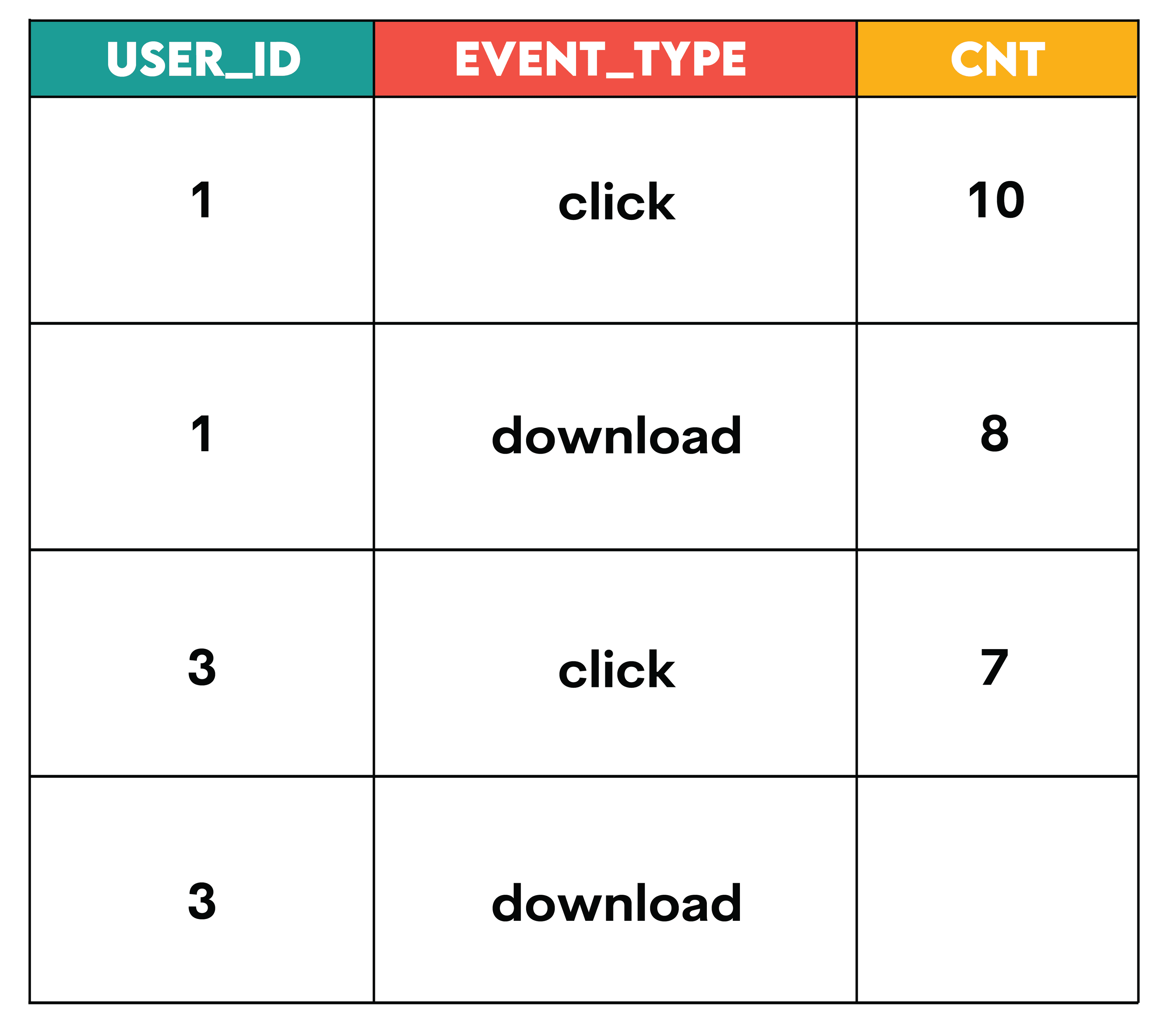
When a particular pivot combination (like event_type = ‘download’ and user_id = 3) exists in the data but the aggregated value (cnt) is missing, SQL will return NULL. One approach is to replace the null value with a 0 (a common default value) if appropriate for the business context. A simple approach to doing so is to take the value and use COALESCE to replace NULL values with a 0.
For example:
SELECT user_ID,
       coalesce(click, 0) AS click_event,
       coalesce(download, 0) AS download_event
FROM
  (SELECT user_ID,
          event_type,
          cnt
   FROM web_events
   WHERE user_ID IN (1,
                     3)) AS source_data PIVOT ((SUM(cnt)
                                                FOR event_type IN (click,
                                                                   download)) AS pivot_table
The output will now be:
Similarly, for string data, there can be different types of formats to indicate NULL values, such as COALESCE(value_column, ‘N/A’).
Note that consistency is the key when understanding and handling missing data/NULL values. 0 is just one example of a default value that can be assigned when data is missing. Another approach would be to understand the type of missing data and then assign a default value accordingly.
Note that the values you chose will be heavily dependent on the business context. As an example,
No data recorded → replace with 0
Unclassified entries → replace with <UNKNOWN>
Incomplete responses → replace with MISSING
2. Handling Missing Categories or Columns
Sometimes a column doesn’t appear at all because that category doesn’t exist in the source data. This is a very common use case when doing retention analysis. If there are specific weeks when no users started or churned, it may happen that the specific week doesn’t exist in the source data.
To explain the concept, let’s choose a simple example of regional sales:
Instead of showing just North and South regions, I want to show all 4 regions, i.e., North, South, East, and West, in my pivoted output.
1) Leverage IN Clause: To fix this problem, we can explicitly define columns in the IN clause of the PIVOT statement.
PIVOT (
    SUM(sales)
    FOR Region IN (North, South, East, West)
) AS pivot_table
This forces all regions to appear even when East and West have no data.
2) Define the regions that you want in the final output in a regions table (sometimes we refer to such tables as dimension tables) and then join the data with the sales table. This ensures that all regions show up.
SELECT r.region, s.sales
FROM regions r
LEFT JOIN sales_data s ON r.region = s.region

Now, you can do something like the below. For each of the regions, the sales/revenue can be imputed as 0 with the help of `COALESCE()`.

SELECT
    region,
    COALESCE([East], 0) AS East_Sales,
    COALESCE([West], 0) AS West_Sales
FROM pivoted_sales;
Multi-Aggregate Pivots and Multiple Measures
Sometimes you may want to have multiple types of aggregations in the columns that you reshape from rows to columns. From the same example of regional sales above, you may want to pivot the data and show both the sum and average sales for each category as columns.
In this case, the approach would be to write two different PIVOT statements and then JOIN or UNION the data together, depending on how you want it displayed in the final output.
Let’s take a look at a similar hypothetical example with this regions table:
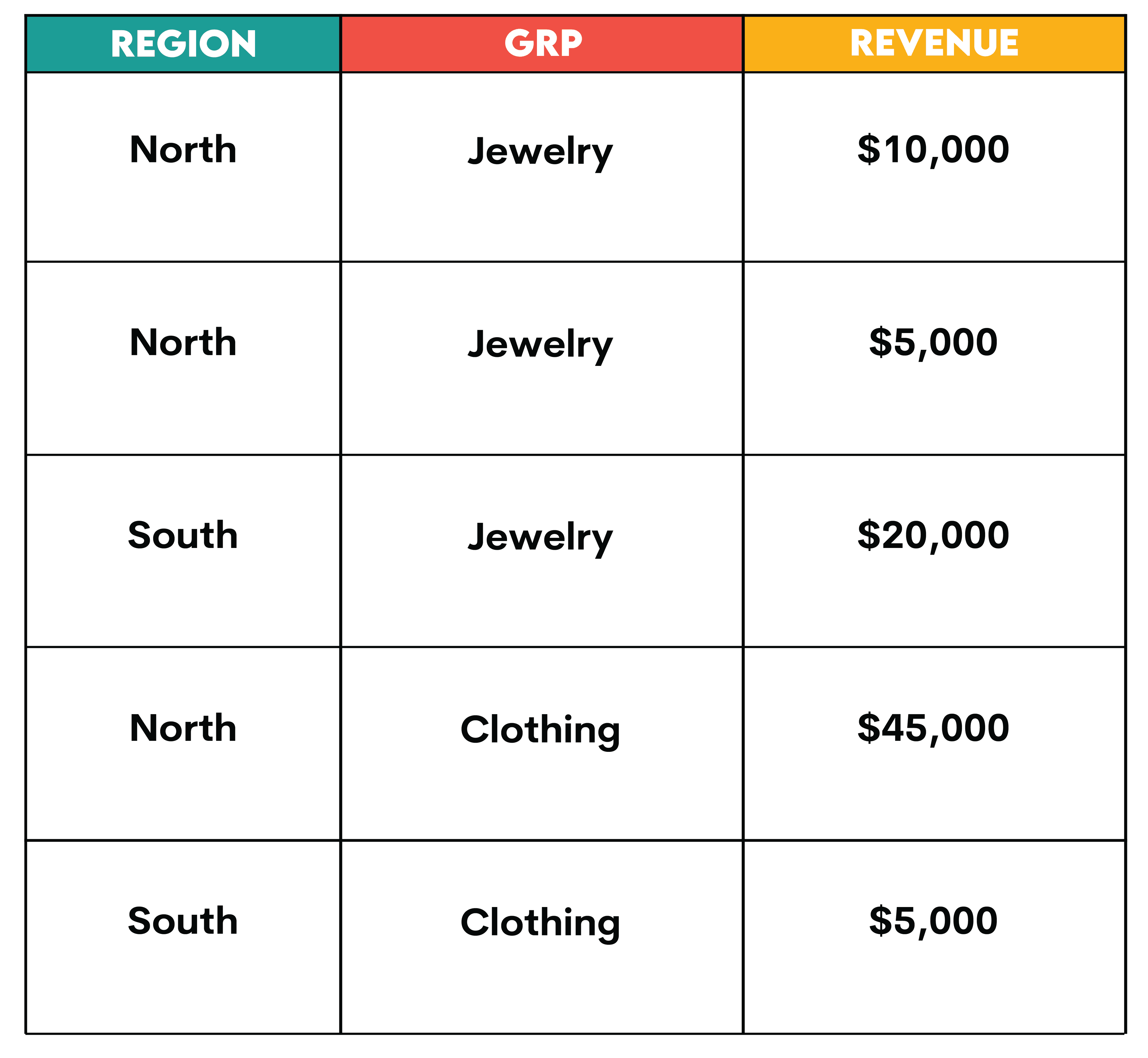
Suppose you wanted to reshape this table into the output shown below. This involves reshaping the unique categories in the grp column from rows to columns and showing both the totals and the averages. This means that you will do two different aggregations (multi-aggregation) i.e., SUM and AVG, respectively.
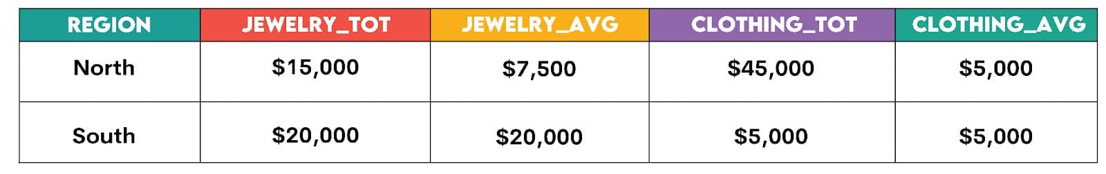
Since PIVOT has some limitations, the approach to doing multi-aggregation is demonstrated in the 3 steps below:
- Pre-aggregate the data and create rows
- Union the data, which is a neat trick to UNPIVOT the data. You will learn more about unpivoting the data once you go through the examples further in this article
- Pivot the rows into columns
WITH base AS
  (SELECT region,
          grp,
          SUM(revenue) AS tot_revenue,
          AVG(revenue) AS avg_revenue
   FROM regions
   GROUP BY region,
            grp)
SELECT region,
       [jewelry_tot],
       [jewelry_avg],
       [clothing_tot],
       [clothing_avg]
FROM
  (SELECT region,
          grp+ '_tot' AS metric,
          tot_revenue AS value
   FROM base
   UNION ALL SELECT region,
                    grp+ '_avg' AS metric,
                    avg_revenue AS value
   FROM base) AS base2 PIVOT (SUM(value)
                              FOR metric IN ([jewelry_tot],
                                             [jewelry_avg],
                                             [clothing_tot],
                                             [clothing_avg])) AS pivot_table
ORDER BY region
Now that we are aware of the approach to creating pivots in SQL, one other approach is Dynamic Pivoting. This is most useful when you don’t know the number of columns that will result once you reshape the data from rows to columns.
Dynamic Pivoting (When the Pivot Columns Aren’t Known Upfront)
In this section, we’ll discuss two approaches to dynamic pivoting:
1. Using CREATE TABLE + PIVOT + IN
One extremely simple approach would be to determine the column that will contain the categories that you want to reshape from long to wide format, and then obtain the distinct list of categories before even applying the PIVOT condition.
For the example that was discussed above (https://platform.stratascratch.com/coding/2047-total-monatery-value-per-monthservice), one way to find the service names would be to just select the distinct list of service names. These service_names can then be input in the IN clause of PIVOT, the way we showed earlier.
CREATE TABLE IF NOT EXISTS tmp_service_names AS
 (SELECT DISTINCT service_name
  FROM  uber_orders)
Once you know the list of service names, the PIVOT + IN part can be executed the same way as I have shown before:
PIVOT (SUM(monetary_value)
                 FOR service_name IN (Uber_BOX,
                                      Uber_CLEAN,
                                      Uber_FOOD,
                                      Uber_GLAM,
                                      Uber_KILAT,
                                      Uber_MART,
                                      Uber_MASSAGE,
                                      Uber_RIDE,
                                      Uber_SEND,
                                      Uber_SHOP,
                                      Uber_TIX)) AS pivot_table
2. Using Stored Procedures
The more advanced approaches require the use of stored procedures in SQL Server. Rather than focusing on all the nuances of the code, let’s look at the fundamental steps involved:
There are primarily three steps involved in this process:
- Identify the list of service names and set a variable for it
- Set a variable for the pivot operation
- Execute the pivot by calling the variable
The details are shown below:
Step 1: Identify the list of service names and set a variable for it
DECLARE @service_list NVARCHAR(MAX)
SELECT @service_list = STRING_AGG(QUOTENAME([service_name]), ',') WITHIN GROUP (ORDER BY [service_name])
FROM (SELECT DISTINCT [service_names] FROM uber_orders WHERE status = ‘completed’) AS services;
- DECLARE @service_list - We set a string variable
- SELECT @service_list…. - Here, we are basically using the string_agg function in SQL to concatenate all the service_names and the QUOTENAME function to escape special characters
- SELECT DISTINCT [service_names] FROM uber_orders – This is us simply identifying the unique service names
Once this is built, then the next steps are basically setting the variable for the pivot and executing the pivot.
Step 2: Set a variable for the pivot operation and write out the pivot operation
DECLARE @service_pivot NVARCHAR(MAX);
SET @service_pivot = N ‘SELECT month(order_date) AS MONTH,  ‘+ @service_list + ‘ FROM uber_orders where status = ‘completed’ PIVOT ( SUM(monetary_value) FOR service_name IN ( ‘ + @service_list + ‘ )) AS final_pivot ORDER BY Month’;
Step 3: Execute the pivot by calling the variable
EXEC(@service_pivot)
This approach is helpful when working with extremely large data where the no. of categories may become very large or when these categories are not known to begin with.
Emulating Pivot with Case Statements & Conditional Aggregation
One thing to keep in mind is that the PIVOT clause doesn’t work in all dialects. For example, in Stratascratch’s most commonly used SQL dialect, PostgreSQL, we don’t have the option to use this clause. Instead, let’s discuss the most universal approach which uses aggregate functions with CASE WHEN statements combined with GROUP BY. The best part is that it’s available in any dialect, and the syntax should be familiar to all SQL practitioners!
Here’s some pseudo-code for reference:
SELECT grouping_col_1,
       grouping_col_2,
       grouping_col_3,
       AGGREGATE_FUNCTION (CASE
                               WHEN condition_1 THEN value_column
                               ELSE NULL
                           END) AS pivoted_col_1,
       AGGREGATE_FUNCTION(CASE
                              WHEN condition_2 THEN value_column
                              ELSE NULL
                          END) AS pivoted_col_2
FROM TABLE_NAME
GROUP BY grouping_col_1,
         grouping_col_2,
         grouping_col_3
Let’s take a look at the main elements of this query:
- The
GROUP BYclause combines rows with the same values for grouping_col_1, grouping_col_2, and grouping_col_3. Visually, this can be thought of as creating distinct groups and is not very different - The
CASE WHENstatements define the pivot conditions. You can use this statement and add filtering conditions using boolean values, e.g.,CASE WHENpivot_condition_1 > 500 - The AGGREGATE_FUNCTION (e.g.,
SUM,AVG,MAX,MIN,COUNT) is applied to the filtered values from theCASE WHENstatements within each group.
Real-World Examples
Now that we are clear on these fundamentals, let’s take a stab at a few real-world examples and interview questions.
Example 1: Using SUM() with Conditional Aggregation
An interview question from Microsoft asks us to find the total number of downloads for paying and non-paying users by date. This is a classic use case of Premium versus Freemium.
Premium vs Freemium
Last Updated: November 2020
Find the total number of downloads for paying and non-paying users by date. Include only records where non-paying customers have more downloads than paying customers. The output should be sorted by earliest date first and contain 3 columns date, non-paying downloads, paying downloads. Hint: In Oracle you should use "date" when referring to date column (reserved keyword).
Here’s a link to the question: https://platform.stratascratch.com/coding/10300-premium-vs-freemium
Tables:
This dataset contains 3 main tables:
- ms_user_dimension: Contains user-level information and whether or not they are paying customers
- ms_acc_dimension: Contains account-level details linked via acc_id
- Ms_download_facts: Contains daily download records for each user
Approach: Before diving into the solution, break this problem into steps to understand how to pivot the data. There are 3 main steps in the approach:
- Group by paying and non-paying users, and aggregate download counts per day
- Filter only the days where non-paying users downloaded more than paying users
- Return the final results in wide format: date, paying_downloads, nonpaying_downloads
Solution: To identify which customer type has more downloads, we need to pivot the paying_customer column from long format to wide format:
To summarize, let’s breakdown the pivot:
- Grouping column: date
- Aggregate function: SUM()
- Pivot conditions: paying_customer = 'yes' and paying_customer = 'no'
- Value column: downloads
Here’s the final output:
| download_date | non_paying | paying |
|---|---|---|
| 2020-08-16 | 15 | 14 |
| 2020-08-17 | 45 | 9 |
| 2020-08-18 | 10 | 7 |
| 2020-08-21 | 32 | 17 |
Example 2: Handling Multiple Categories
Let’s take a look at the Uber question, but this time solve it using CASE WHEN statements and conditional aggregation. Our goal is to find the total monetary value for completed orders by service type for every month. The output is a pivot table with a column for month and columns for each service type.
Total Monetary Value Per Month/Service
Last Updated: June 2021
Find the total monetary value for completed orders by service type for every month. Output your result as a pivot table where there is a column for month and columns for each service type.
Here’s a link to the question: https://platform.stratascratch.com/coding/2047-total-monatery-value-per-monthservice
Tables:
Approach: Before diving into the solution, break this problem into steps to understand how to pivot the data. There are 3 main steps in the approach:
- Filter for completed orders only
- Group by month and aggregate monetary values by service type
- Return the final results in wide format, with each service type as its own column
Solution: To transform service types from rows into columns, we need to pivot the service_name column from long format to wide format using this standard approach:
To summarize, let's breakdown the pivot:
- Grouping column: month (extracted from order_date)
- Aggregate function:
SUM() - Pivot conditions:
service_name = 'Uber_BOX',service_name = 'Uber_CLEAN', etc. (11 distinct services) - Value column: monetary_value
In the above question, as the number of services increases, one thing to consider is whether there is a more efficient way of creating a PIVOT, especially if you aren’t aware of the no. of categories you are dealing with in advance. Here’s where we start exploring dialect-specific options that are available to us.
Example 3: Using CROSSTAB in PostgreSQL
Let’s take a look at the same problem as in Example 2. PostgreSQL's tablefunc extension provides the CROSSTAB() function for pivoting. This is a good alternative to explore since PostgreSQL also doesn’t have the native PIVOT capability. Note: The tablefunc extension must be enabled first.
CREATE EXTENSION IF NOT EXISTS tablefunc
Now let’s take a look at the solution and understand how it works:
SELECT
 *
FROM
 crosstab (
   'SELECT EXTRACT(MONTH FROM order_date)::integer AS month,
           service_name,
           SUM(monetary_value) AS total
    FROM uber_orders
    WHERE status_of_order = ''Completed''
    GROUP BY EXTRACT(MONTH FROM order_date), service_name
    ORDER BY 1, 2',
   'SELECT DISTINCT service_name
    FROM uber_orders
    WHERE status_of_order = ''Completed''
    ORDER BY 1'
 ) AS ct (
   MONTH INTEGER,
   Uber_BOX NUMERIC,
   Uber_CLEAN NUMERIC,
   Uber_FOOD NUMERIC,
   Uber_GLAM NUMERIC,
   Uber_KILAT NUMERIC,
   Uber_MART NUMERIC,
   Uber_MASSAGE NUMERIC,
   Uber_RIDE NUMERIC,
   Uber_SEND NUMERIC,
   Uber_SHOP NUMERIC,
   Uber_TIX NUMERIC
 )
ORDER BY
 MONTH
To summarize, let's breakdown the CROSSTAB pivot:
- First query (source data): Aggregates monetary_value by month and service_name
- Second query (category list): Provides the distinct service names to become columns
- Output specification: Defines the result table structure with the month and all service columns
- Aggregate function: SUM() (applied in the source query)
Once you execute this code, you will get the same result as the previous example.
Example 4: Unpivoting Data
Now that we know how to pivot data, let’s also take a look at how to unpivot, i.e., transform data from wide format back into long format. While SQL Server offers an UNPIVOT function, a more dialect-agnostic approach uses UNION or UNION ALL.
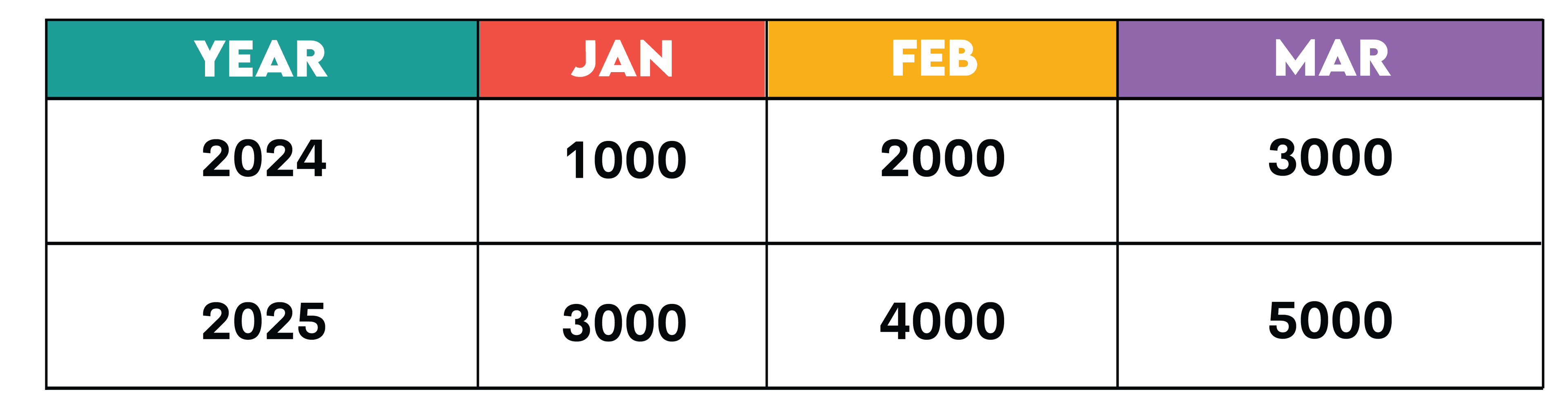
Let’s take a look at this hypothetical example where I have sales for every month in columns, and I want to transform the data into rows. This is also a common use case for time series modeling, where your data needs to be in long format to feed into popular forecasting models.
Example: Unpivot monthly sales data
Original table:
Unpivoting with UNION ALL:
SELECT Year, 'January' AS Month, Jan AS Sales
FROM month_sales
UNION ALL
SELECT Year, 'February' AS Month, Feb AS Sales
FROM month_sales
UNION ALL
SELECT Year, 'March' AS Month, Mar AS Sales
FROM month_sales;
Result:
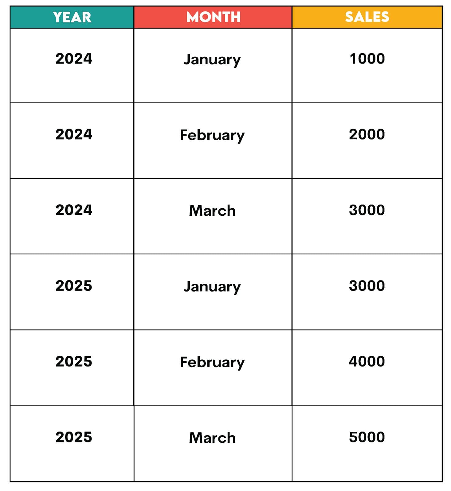
This approach is straightforward, but if you are new to using UNION or UNION ALL, take a look at UNION vs UNION ALL. Note that this approach may be computationally expensive in case the volume of data is large.
A more efficient approach to achieving the same results can be with the use of CROSS JOIN LATERAL (PostgreSQL). You can find more information about the use of lateral with cross joins in the official documentation here.
Here’s the query for unpivoting using this approach.
SELECT YEAR,
       md.month,
       md.sales
FROM month_sales
CROSS JOIN LATERAL (
                    VALUES ('January',
                            Jan), ('February',
                                   Feb), ('March',
                                          Mar)) AS md(MONTH, sales);
In the above approach, there are three main steps:
- The query reads one row from the month_sales table (e.g., YEAR=2024, Jan=1000, Feb=2000, Mar=3000)
- The
VALUESclause takes that one row and creates 3 rows - The
LATERALclause just ensures that the above steps are done for each row in the table
Now that we know how to PIVOT and UNPIVOT the data, let’s look into some best practices to keep in mind for Pivoting in SQL.
Best Practices for Pivoting
When working with large datasets and pivoting operations, keep these principles in mind:
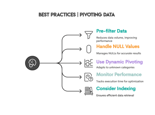
- Pre-filter data: Always filter and reduce data volume before pivoting to improve performance
- Handle NULL values: Understand and appropriately manage NULL values in your aggregations. Very simple techniques, such as using a
COALESCE()function to input 0s instead ofNULLvalues, can be a useful trick to get your results formatted without NULLs. Learn more about COALESCE here! - Use dynamic pivoting: For many or unknown categories, prefer
CROSSTAB()or dive deep into using Dynamic SQL - Monitor performance: Evaluate query execution time and optimize as needed
- Consider indexing: Index on grouping and filtering columns
Pivot in SQL vs Pivot in BI Tools
Pivoting is such a fundamental skill that it can be explored in any tool (Python, SQL, and even BI tools). One question that may come to mind is when to pivot in SQL versus BI tools?
On the job, you will be doing both, but the choice between choosing to pivot in SQL and pivot in BI tools is often dependent on a deep understanding of the use case, data architecture, and the scale that you are dealing with. In my experience, there are several ways to think about the use case involved. Let’s take a look at a few considerations.
Some benefits of pivoting in SQL over BI reporting:
1. Optimizing for Scale: If data is very large, pre-aggregation is likely to reduce the latency of dashboards and ensure that dashboards load quickly. Note that this is critical for executive-friendly dashboards. You have to pull out all the stops when ‘productizing insights’!
2. Fixed/Standard Reporting: If the way you look at data and trends is consistent from week to week and all your filters are pre-aligned, using SQL is likely to be more efficient than using BI tools. This is typically more common for established products with a steady rhythm of business performance monitoring.
Some benefits of pivoting/data reshaping in BI reporting over SQL:
3. Flexible BI Reporting: This is a common need to support self-serve analytics at scale. Imagine you are a data science lead for a product that is being managed by multiple teams and functions (not uncommon in large organizations). Enabling self-serve is a critical aspect where you can load a flat dataset into tools (E.g., Tableau) and create some basic visualizations. Users of these self-serve dashboards can then drag and drop fields to slice and dice key metrics and evaluate opportunities. In this scenario, pivoting in BI tools may be a more flexible option.
4. Technical Skills: BI reporting is easier for many non-technical functions to explore the data and answer questions with high velocity. Since BI reporting doesn’t require writing code, data can be decentralized among a larger number of teams with this capability.
Conclusion
Pivoting data in SQL is an essential skill for data professionals. Whether you use conditional aggregations or dialect-specific functions like PIVOT() and CROSSTAB(), mastering these techniques enables you to effectively reshape data for analysis, build features for machine learning models, and communicate insights clearly. Choose the approach that best fits your use case. Simply, conditional aggregation for simplicity, or native pivot functions for cleaner syntax and better performance, or dynamic SQL in case of many categories, and if the categories are not known upfront.
Frequently Asked Questions (FAQs)
Does every SQL database support the
PIVOTkeyword?
No, SQL Server, Oracle, Snowflake, BigQuery are a few dialects that support the PIVOT keyword, but others like PostgreSQL, MySQL don’t. Be sure to check the documentation of the SQL dialect you are using. For interview preparation, focus on the logic and dialect-agnostic approaches so that you can implement the logic in any dialect.
What is the difference between
PIVOT()andUNPIVOT()in SQL?
PIVOT() is transforming the data from long format to wide format (rows to columns), and UNPIVOT() is just the opposite (columns to rows).
How do I create a dynamic pivot in SQL?
We have discussed two approaches in this article using dynamic SQL. The most flexible approach is to use Dynamic Pivoting with the help of stored procedures.
There are primarily three steps involved in this process:
- Identify the list of service names and set a variable for it
- Set a variable for the pivot operation
- Execute the pivot by calling the variable
Can I pivot without aggregation in SQL?
While you still need to use aggregate functions as a part of the syntax, if there is only 1 value per row, these aggregate functions don’t really aggregate but rather just pick the single value that exists.
Which is better: pivoting in SQL or in BI tools like Power BI or Tableau?
It depends on the use case. For more flexibility and self-serve analytics, choose pivoting in Power BI or Tableau. Alternatively, if you are handling extremely large datasets and have a set format for reporting, it is better to pre-aggregate and pivot your data in SQL for efficient processing and reducing latency in dashboards.
How do I replace NULL values after pivoting?
A simple coalesce function should do the trick to replace NULL values with 0. Always sample your records to develop intuition about what to expect after you pivot the data.
Share