Basic Types of Statistical Tests in Data Science

Navigating the World of Statistical Tests: A Beginner’s Comprehensive Guide to the Most Popular Types of Statistical Tests in Data Science

In the midst of concepts and buzzwords like machine learning, deep learning, clustering, anomaly detection, and so on in the world of data science, statistical tests are a very underrated, yet important concept that every Data Scientist should know.

A knowledge about statistical tests enables us to report an accurate insight about the data. Every Data Analyst or Data Scientist can create a report that tells that product A is more impactful than product B just by looking at the number in the data. However, the main and more important question is, can we trust the result that comes out from our data?

Hypothesis Testing

As we might know, when we infer something from data, we make an inference based on a collection of samples rather than the true population. The main question that comes from it is: can we trust the result from our data to make a general assumption of the population? This is the main goal of hypothesis testing.

There are several steps that we should do to properly conduct a hypothesis testing:

• First, form our null hypothesis and alternative hypothesis.
• Set our significance level. The significance level varies depending on our use case, but the default value is 0.05.
• Perform a statistical test that suits our data.
• Check the resulting p-Value. If the p-Value is smaller than our significance level, then we reject the null hypothesis in favor of our alternative hypothesis. If the p-Value is higher than our significance level, then we go with our null hypothesis.

So far you’ve seen the general approach on how to conduct hypothesis testing. However, everything up to now might seem a little abstract for you. Given our data, how can we properly form a null hypothesis and an alternative hypothesis? Which type of statistical test should we perform?

In the following section, we’re going to discuss how we can formulate our null hypothesis and alternative hypothesis.

Null Hypothesis vs Alternative Hypothesis

Null hypothesis and alternative hypothesis are two hypotheses that are conflicting with each other. Our task is to choose which type of statistical test we should take: null or alternative?

Null Hypothesis

Null hypothesis is the accepted status quo. It’s the default value. It states that nothing happened, no association exists, no significant difference between the mean or the proportion of our sample and the population.

As an example, let’s say we have gathered quite a few sample data about the proportion of men and women in New York. Next, we want to know if there is a difference between the men-women proportion in our data in comparison with the actual men-women proportion in the whole of New York.

The formulation of null hypothesis will be something like this:

“There is no significant difference between the men-women proportion of our data and the general population in New York”

It assumes that everything is fine.

Alternative Hypothesis

The alternative hypothesis is the complete opposite of the null hypothesis. It states that there is something going on, there is a significant difference between the mean or the proportion of our sample and the population.

There are three different variations of alternative hypothesis that you should know:

Two-sided hypothesis

Two-sided hypothesis can be used when we just want to know if there is a significant difference between pothe mean or proportion of our sample data with the population.

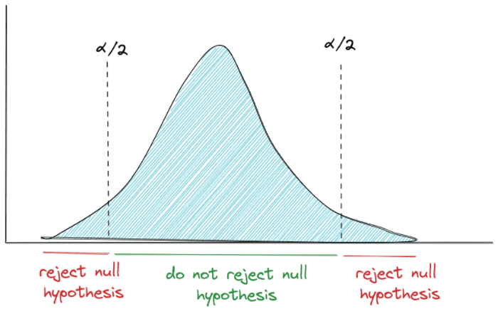
Let’s use the example from null hypothesis to illustrate how we can formulate two-sided alternative hypothesis:

“There is a significant difference between the men-women proportion of our data and the general population in New York”

Left-sided hypothesis

Left-sided hypothesis can be used when we want to know if the mean or proportion of the population is smaller than our sample data.

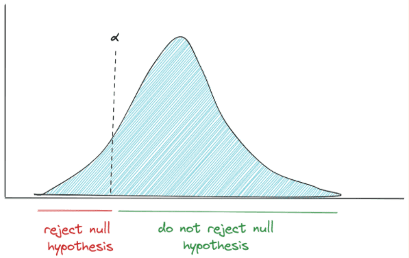
Considering the example that we’ve used so far, below is the formulation of left-sided hypothesis:

“The men-women proportion in the general population in New York is less than the men-women proportion of our data.”

Right-sided hypothesis

Right-sided hypothesis can be used when we want to know if the mean or proportion of the population is larger than our sample data.

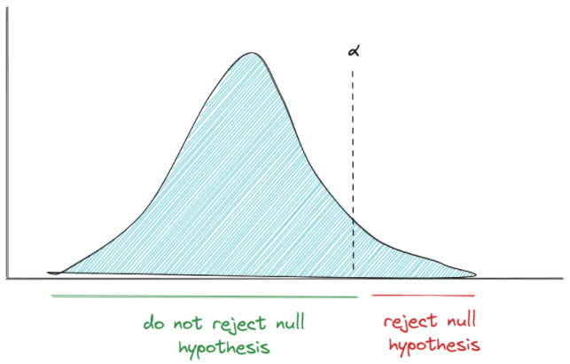
If we use the example that we’ve used above, we can formulate the right-sided hypothesis as follows:

“The men-women proportion in the general population in NewYork is larger than the men-women proportion of our data.”

Null Hypothesis vs Alternative Hypothesis: Which Statistical Test to Choose?

Since the null hypothesis is always going to be our default value, we cannot ‘accept’ the null hypothesis. We can either reject the null hypothesis in favor of the alternative hypothesis, or go with our null hypothesis.

Now, to know whether or not we should reject the null hypothesis, it depends on two factors:

• The significance level
• The p-Value

We can set the value of significance level in advance, for example 0.05. Meanwhile, we need to conduct test statistics in order to find the p-Value.

The general idea is that if the resulting p-Value is less than our significance level, we reject the null hypothesis. If the p-Value is larger than our significance level, we go with our null hypothesis.

The problem is, there are various test statistics out there. Which type of statistical test we should apply is totally dependent on our use case and data. So the natural question that comes next is, which type of statistical test should we choose considering the problem and data that we have?

To answer this question, we’re going to show you different types of statistical tests available out there and when you’re going to need each of them with one example dataset as our use case. So, let’s take a look at the dataset first.

Dataset to demonstrate the use of each type of statistical test

To demonstrate the use of each type of statistical test, of course we need data for it. In this article, we’re going to use a student dataset. Below is the snapshot of what the dataset looks like:

import pandas as pd
df = pd.read_scv('students.scv')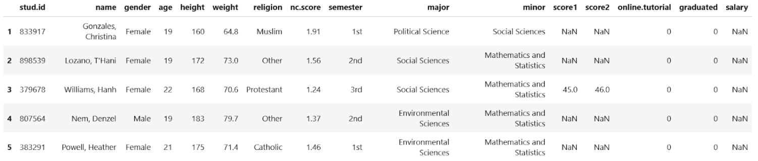

Particularly, we are interested in the following variables throughout this article:

• gender: the gender of the students -> categorical variable
• weight: the weight of the students -> continuous variable
• religion: the religion of the students -> categorical variable
• major: the study major of the students -> categorical variable
• score1: the grades of the students for the first exam -> continuous variable
• score2: the grades of the students for the second exam -> continuous variable
• online.tutorial: whether the students take an online tutorial between the first exam and the second exam -> categorical variable
• salary: the salary of the students who graduated already -> continuous variable

As you can see, we have a combination of continuous and categorical variables in our dataset. These combinations of variables will help us to better understand which statistical tests that we need to conduct for our use case.

Most Popular Types of Statistical Tests in Data Science

Now that we know the data that we will work with in this article, let’s start with the first statistical test type, which is the Z-test for population mean.

Z-test for Population Mean

Z-test for population mean is the simplest statistical test type out there, which makes it a good subject for us to start learning about hypothesis testing. As the name suggests, Z-test is a statistical test to compare the average of sample mean against the population mean.

To properly conduct this test, we need to make sure that our data fulfills the prerequisites as follows:

• The variable in our data is a continuous variable and follows a normal distribution or
• We have a large sample size for our variable
• The sample is randomly selected from its population
• The population standard deviation is known

The last point there, which is the population standard deviation must be known, is almost never fulfilled in real-life because normally we don’t know the standard deviation of the population.

Below is the general equation of a Z-test for population mean

where Z is the Z-score, x_bar is the sample mean, μ is the population mean, σ is the standard deviation of population and n is the number of samples.

Example Use Case:

In this statistical test, we’re going to use the weight variable from our dataset.

We want to know: Is there any difference between the average weight of European students and European adults, given that we know the average and standard deviation of European adults’ weight?

This is the use case that can be answered with the Z-test because we fulfill the following conditions:

• We have gathered a large sample data
• Weight is a continuous variable

But there is a catch here. How do we know the population mean and standard deviation?

A research conducted by Walpole et al. stated that the average weight of European adults is 70.8 kg. However, we still don’t know its standard deviation. Hence, for the sake of demonstration, we’re going to assume that the population standard deviation is equal to sample standard deviation.

Now we can form our null and alternative hypothesis:

• Null hypothesis: the average weight of European students (sample) is equal to the average weight of European adults (population).
• Alternative hypothesis: the average weight of European students (sample) is different from the average weight of European adults (population).

Since we formulate the alternative hypothesis as above, then it means that we perform two-sided hypothesis testing.

Let’s say that our significance value is 0.05. Next, we can compute the Z-score and p-Value by using a statistical library in Python or R. In this article, we’re going to use the statsmodels library in Python to conduct the Z-test and compute the p-Value.

from statsmodels.stats.weightstats import ztest

test_stats, p_value = ztest(x1=df['weight'], value=70.8, 
alternative='two-sided')

print(p_value)
output: 4.0517857849264745e-118

As you can see from the code snippet above, the p-Value that we got is 4.05e-118, which is way smaller than our significant value. Hence, we conclude that our data provides strong evidence to reject the null hypothesis at significance level of 0.05.

One-Sample t-test for Population Mean

One-sample t-test is the more general version of the Z-test. As mentioned previously, what makes the Z-test difficult to implement in real-life is its assumption about population standard deviation that we need to fulfill. In real-life, oftentimes we don’t know the population standard deviation. And this is where we can conduct one sample t-test.

To properly conduct this test, we need to make sure that our data fulfills the following condition:

• The variable in our data is a continuous variable and follows a normal distribution or
• We have a large sample size
• The sample is randomly selected from its population

Below is the equation of one sample t-Test:

where t is the t-statistic, x_bar is the sample mean, μ is the population mean, s is sample’s standard deviation, and n is the number of samples.

Example use case:

In this use case, we’re going to use the same variable as the one from Z-test above, which is the weight variable.

We want to know: Is there any difference between the average weight of European students and the average weight of European adults, given that we didn’t know the standard deviation of the weight of European adults?

The null and alternative hypothesis are similar with the one from z-Test for population mean above.

• Null hypothesis: the average weight of European students is similar to the average weight of European adults
• Alternative hypothesis: the average weight of European students is different from the average weight of European adults.

Since we formulate the alternative hypothesis as above, then it means that we perform two-sided hypothesis testing.

Let’s say that we set the significance value to be 0.05. Next, we can compute the test statistics and p-Value with statistical libraries available out there. In this case, we’re going to use Scipy library in Python to compute the test statistic and p-Value.

from scipy.stats import ttest_1samp

test_statistic, p_value = ttest_1samp(df['weight'], popmean=70.8, 
alternative='two-sided')

print(p_value)
output: 1.6709961011966605e-114

As you can see, the p-Value that we got is extremely small, which is 167e-114. This means that at 0.05 significance level, our data provides very strong evidence to reject the null hypothesis, i.e the average weight of European students is indeed different from the average weight of European adults.

Paired t-Test

In the previous section, we have seen how we can conduct a statistical test when we want to compare the means of our sample with the general population.

With paired t-tests, the goal is different compared to one-sample t-test. Instead of comparing our sample with the population, we want to compare two different conditions on the same variable and then check whether there is any significant difference between the two conditions.

To properly conduct this test, we need to make sure that our data fulfill the following conditions:

• The variable in our data is a continuous variable and follows a normal distribution or
• We have a large sample size
• The sample is randomly selected from its population

Below is the general equation of t-statistic for paired t-tests.

where t is the t-statistic, d is the difference between two conditions and n is the number of samples.

Example use case:

In this use case, we’re going to use three variables from our dataset: score1, score2, and online.tutorial.

We want to know: Is there any difference between the students’ grades before and after taking an online learning tutorial? Is online learning tutorial actually helps the students to improve their exam’s grades?

This is the question that we can solve with paired t-tests. Now let’s prepare our data.

df_score = df[(df['online.tutorial'] == 1) & (df['score1'].notnull()) & 
(df['score2'].notnull())][['name','score1','score2','online.tutorial']]

First, as usual, we set our significance level, which in this case let’s set it to 0.05. Next, we form our null hypothesis and alternative hypothesis as follows:

• Null hypothesis: the average grades before and after taking an online learning tutorial is the same.
• Alternative hypothesis: the average grades after taking an online learning tutorial (score2) is higher than before (score1).

Notice that with the way we formulate the alternative hypothesis, we’re conducting a left-sided hypothesis. Now let’s compute the t-statistics by plugging in values to paired t-tests equation above:

from scipy.stats import ttest_rel

test_statistic, p_value = ttest_rel(df_score['score1'], 
df_score['score2'], alternative='less')

print(p_value)
output: 8.946942058314536e-77

As you can see, in the end the p-Value is very small, which means that we can say that the average student’s grades after taking an online tutorial is indeed higher than before. At a significance level of 0.01, we reject the null hypothesis in favor of the alternative hypothesis.

But sometimes we may have the following hypothesis: probably the second exam is easier than the first exam, thus the students are performing better in the second exam. To prove this hypothesis, we’re going to take the data from students who didn’t take the online tutorial and compare the grades of their first and second exam.

df_score_no_tutorial = df[(df['online.tutorial'] == 0) & 
(df['score1'].notnull()) & (df['score2'].notnull())]
[['name','score1','score2','online.tutorial']]

This is our null and alternative hypothesis:

• Null hypothesis: among students who didn’t take an online tutorial, the average grades of the first exam is the same as the second exam.
• Alternative hypothesis: among students who didn't take an online tutorial, the average grades of the second exam is higher than the first exam.

From the way we formulate our hypothesis, we’re conducting a left-sided hypothesis. With Scipy, we can compute the p-Value as you can see below:

from scipy.stats import ttest_rel

test_statistic, p_value = ttest_rel(df_score_no_tutorial['score1'], 
df_score_no_tutorial['score2'], alternative='less')

print(p_value)
output: 0.7232359247303264

As you can see, the p-Value for this case is 0.722, which means that it is higher than our significance level. Hence, we can’t reject our null hypothesis and deny the hypothesis that the students’ grades improvement is due to easier exams.

Two-Sample t-Test

So far, we have covered the case where we want to infer one variable. In some cases, what we want to do instead is to compare two independent variables and observe whether there is any significant difference between two variables. For this purpose, we can use a two-sample t-test.

To properly conduct this test, we need to make sure that our data fulfills the following conditions.

• Two variables are independent
• Two variables are randomly selected from their population
• Two variables are continuous variables and have normal distribution distribution
• The result of the statistical test will be more robust or reliable if the sample size of two variables are the same.

Below is the equation of two sample t-test:

where the index 1 and 2 denote our first and second variables, t is the t-statistic, x_bar is the sample mean, s is sample’s standard deviation, and n is the number of samples.

The t-statistic that comes out from the equation above measures the mean and standard error difference between two samples.

Example use case:

In this use case, we’re going to use two variables from our dataset: gender and salary.

Now we want to know: Is there any difference in the average salary between university graduates in relation to gender (men vs women).

This use case can be answered by conducting two sample t-tests. One variable contains the salary of male graduates and another contains the salary of female graduates.

df_male = df[(df['gender'] == 'Male') & 
(df['salary'].notnull())].sample(n=500)[['name', 'gender','salary']]

df_female = df[(df['gender'] == 'Female') & 
(df['salary'].notnull())].sample(n=500)[['name', 'gender','salary']]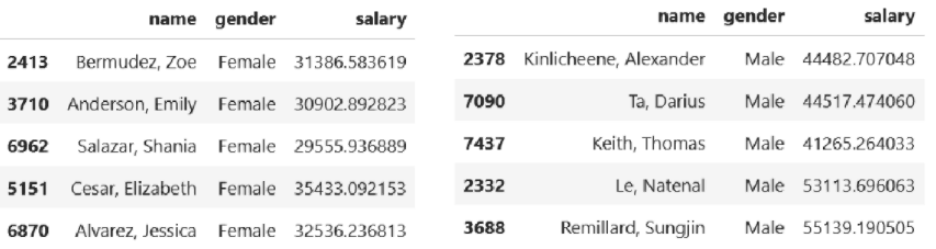

Next we can form our null and alternative hypothesis as follows:

• Null hypothesis: the average mean salary of male graduates is equal to the average mean salary of female graduates.
• Alternative hypothesis: the average mean salary of male graduates is higher than the average mean salary of female graduates.

Notice that because of the way we formulate the alternative hypothesis, this means that we conduct a right-sided hypothesis.

Let’s define the significance level for this use case to 0.01. Same as before, we need to compute the test statistic and p-Value by using a statistical library. We’re going to use Scipy for this test.

from scipy.stats import ttest_ind

test_statistic, p_value = ttest_ind(df_male['salary'], df_female['salary'], 
alternative='greater')

print(p_value)
output: 2.0579274970768232e-69

As you can see from the result of code snippets above, the resulting p-Value is very small. Hence even if we set the significance level to 0.01, our data provides very strong evidence that the mean salary of male graduates is indeed higher than the mean salary of female graduates. Hence, we reject the null hypothesis.

ANOVA

You’ve seen previously that with a two-sample t-test, we can compare the means of two groups. Now the question is, what if we want to compare the means of more than two groups? In this case, we’ll use a different type of statistical test. We can use ANOVA.

There are 3 different types of ANOVA:

• One-way ANOVA, if we have just one independent variable.
• Two-way ANOVA, if we have two independent variables.
• N-way ANOVA, if we have n independent variables.

To properly conduct ANOVA, we need to fulfill the same requirements as two-sample t-test, such as:

• The variables are independent
• The variables are randomly selected
• The variables have normal distribution
• The result of statistical test will be more robust if the sample size of variables are similar

Below is the general equation of ANOVA:

where f is the f-statistic, MSB is the mean square between groups, and MSW is the mean square within groups. Computing MSB and MSW is a very tedious task if you want to do it by hand. Hence, normally we use a statistical library to conduct an ANOVA test.

Example Use Case:

In this use case, we’re going to use two variables from the dataset: major and salary.

Now we want to know: Is there any difference in the average salary between university graduates in relation to their study major?

This use case is very similar to the one from a two-sample t-test. However, in the two-sample t-test, we compare salary with gender and gender only consists of two groups: male and female. Meanwhile, here we compare the salary and study major. Study major itself has 6 groups.

The use case is also an example of one-way ANOVA, since we only have one independent variable (study major). Meanwhile, if we want to test whether there is any difference in the average salary between university graduates in relation to their study major and gender, then we can implement two-way ANOVA. This is because in this case, we have two independent variables (study major and gender).

Let’s prepare our data first. We’re just going to take 200 samples from each group of study majors.

df_biology = df[(df['major'] == 'Biology') & 
(df['salary'].notnull())].sample(n=200)[['name','major','salary']]

df_economics = df[(df['major'] == 'Economics and Finance') & 
(df['salary'].notnull())].sample(n=200)[['name','major','salary']]

df_environmental = df[(df['major'] == 'Environmental Sciences') & 
(df['salary'].notnull())].sample(n=200)[['name','major','salary']]

df_mathematics = df[(df['major'] == 'Mathematics and Statistics') & 
(df['salary'].notnull())].sample(n=200)[['name','major','salary']]

df_politics = df[(df['major'] == 'Political Science') & 
(df['salary'].notnull())].sample(n=200)[['name','major','salary']]

df_social = df[(df['major'] == 'Social Sciences') & 
(df['salary'].notnull())].sample(n=200)[['name','major','salary']]

Now we can form our null and alternative hypothesis as follows:

• Null hypothesis: there is no significant difference of average salary between university graduates in relation to their study majors.
• Alternative hypothesis: there is a significant difference of average salary between university graduates in relation to their study majors.

Next, let’s set the significance level. For this use case, let’s use 0.05 as our significance level. Same as before, we’re going to use Scipy library to conduct the ANOVA test and compute the resulting p-Value.

from scipy.stats import f_oneway

f_stats, p_value = f_oneway(df_biology['salary'], df_economics['salary'], 
df_environmental['salary'] , df_mathematics['salary'], df_politics['salary'], 
df_social['salary'])

print(p_value)
output: 1.4642372015448516e-144

As you can see, the resulting p-Value is very small in comparison with our significance level. Thus, our data provides strong evidence that there is a significant difference of average salary between university graduates in relation to study majors. In other words, we reject our null hypothesis.

Chi-Square Goodness-of-Fit (GoF)

So far, we have seen the types of statistical tests that are relevant if we have continuous data. You might ask, what if my variable is a discrete or a categorical? If we have a categorical variable, then we need to apply a different approach to our statistical test, and Chi-Square Goodness-of-Fit (GoF) is one of them.

The basic idea of Chi-Square GoF is to compare the observed frequencies of a sample with its expected frequencies. In order to conduct this test, we need to make sure that our data fulfills the following prerequisites:

• The data should be categorical and not continuous
• The sample data is large enough in each category. As a rule of thumb, there should be at least 5 samples in each category
• The sample is randomly selected

Below is the formula of Chi-Square GoF:

where O is the observed frequency in each group, E is the expected frequency in each group, and k is the total number of groups.

The general step that we need to do to conduct Chi-Square GoF is similar to what we’ve seen previously. The test statistic should be computed and then the resulting p-Value will be used to decide whether or not we should reject the null hypothesis.

Example use case:

In this use case, we’re going to use one variable from the dataset, which is religion.

Now we want to know: is there any difference between religion distribution among students compared to religion distribution among European adults?

When we conduct a Chi-Square GoF test, we need to know three additional data: observed frequency, relative frequency, and expected frequency.

Observed frequency is just the number of samples in each group, as you can see below:

df_sample = df.sample(n=500)

df_obs_freq = pd.DataFrame({'observed_freq' : 
df_sample.groupby(['religion']).size()}).reset_index()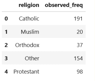

Meanwhile, relative frequency is the proportion of each group in the population. For the sake of this article, let’s say that the Catholic population in the Europe is 48%, Muslim 2%, Orthodox 8%, Protestant 12%, and other religion 30%.

Based on the information above, we can set the relative frequency as below:

religion = ['Catholic', 'Muslim', 'Orthodox', 'Other', 'Protestant']
rel_freq = [0.48, 0.02, 0.08,0.30, 0.12]

df_rel_freq = pd.DataFrame({'religion' : religion, 'rel_freq': rel_freq})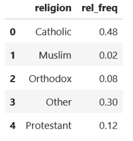

Now, expected frequency is the multiplication of relative frequency and the total number of our samples. Hence,

df_exp_freq = df_obs_freq.merge(df_rel_freq, on='religion')
df_exp_freq['expected_freq'] = df_exp_freq['rel_freq']*500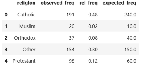

As you can see, now we have observed frequency and expected frequency in each group and we can use these values to conduct the Chi-Square GoF test.

But before that, as usual, we need to set our significance value for this case, which will be 0.01 and then form our hypothesis as follows:

• Null hypothesis: The religion distribution among students is similar to the religion distribution among European adults
• Alternative hypothesis: The religion distribution among students is different compared to the religion distribution among European adults.

Now let’s use Scipy library from Python to conduct this test.

from scipy.stats import chisquare

test_statistic, p_value = chisquare(df_exp_freq['observed_freq'], 
df_exp_freq['expected_freq'])

print(p_value)
output: 5.2921362560681225e-09

The resulting p-Value is very small, indicating that even at significance level of 0.01, our data provides strong evidence that the religion distribution among students is different compared to the religion distribution among European adults. Hence, we reject the null hypothesis.

Chi-Square Independence Test

Although the name of this statistical test is similar to the previous test, the Chi-Square independence test has a different purpose compared to Chi-Square GoF. We use indepence test when we want to observe whether there is an association between two discrete or categorical variables.

To properly conduct this statistical test, we need to make sure that our data fulfills the following conditions:

• The two variables should be discrete or categorical variables
• The sample size of both categories should be large enough. As a rule of thumb, there should be 5 samples in each category
• The samples from both categories are randomly selected.

Below is the general equation of Chi-Square independence test:

where r and c are our two categorical variables.

Example use case:

In this use case, we’re going to use two variables from the dataset: major and gender.

Now we want to observe: Is there any association between gender and study major? In other words, do female students prefer a particular study major in comparison with male students?

The most common practice when we’re dealing with Chi-Square independence test is creating a contingency table of our categorical variables, as you can see below:

df_major = pd.crosstab(df['major'], df['gender'])

Now that we have a contingency table as above, we are ready to conduct the Chi-Square independence test.

But before that, we should set our significance level, which in our case will be 0.05. Next,we formulate our null hypothesis and alternative hypothesis as follows:

• Null hypothesis: there is no association between gender and study major of the students.
• Alternative hypothesis: there is an association between gender and study major of the students.

Now we can compute the resulting p-Value with Scipy library from Python as follows:

from scipy.stats import chi2_contingency

test_statistic, p_value, x, c = chi2_contingency(df_major)

print(p_value)
5.501737149286338e-187

As you can see, the resulting p-Value is very small. This means that at 5% significance level, our data provides strong evidence that there is an association between gender and study major. Hence, we reject the null hypothesis.

Conclusion

We hope that this article is useful for you as an introduction to the most popular types of statistical tests in data science out there. As you already know from the discussion in this article, there are a lot of statistical tests that will help you to make sense of your data. It is our task to identify which statistical test would be the most appropriate for us depending on the problem that we want to solve.

Also, check out our post A Comprehensive Statistics Cheat Sheet for Data Science Interviews which covers topics that focus more on statistical methods rather than fundamental properties and concepts, meaning it covers topics that are more practical and applicable in real-life situations.