Whole Foods Market Data Science Interview Question Walkthrough

Categories:
 Written by:
Nathan Rosidi
Welcome to another tutorial on solving data science interview questions. This time our interview question is from Whole Foods Market.
Whole Foods Market is a chain of supermarkets that sells natural and organic foods, founded in 1980 in Austin, Texas.
This is one of the hard level data science interview questions. The question came up at the Whole Foods Market interviews.
It’s a question that requires knowing data aggregation with the groupby() function.
This data science interview question involves analyzing customer data to understand their spending habits and segmenting them into different groups based on their activity.
We will first explore the data set, outline our approach to solving the problem, and then walk you through coding step-by-step. By the end of this tutorial, you should better understand how to use these powerful functions in your own data analysis projects.
Whole Foods Market Data Science Interview Question
WFM Brand Segmentation based on Customer Activity
Last Updated: June 2021
WFM would like to segment the customers in each of their store brands into Low, Medium, and High segmentation. The segments are to be based on a customer's average basket size which is defined as (total sales / count of transactions), per customer.
The segment thresholds are as follows:
- If average basket size is more than $30, then Segment is “High”.
- If average basket size is between $20 and $30, then Segment is “Medium”.
- If average basket size is less than $20, then Segment is “Low”.
Summarize the number of unique customers, the total number of transactions, total sales, and average basket size, grouped by store brand and segment for 2017.
Your output should include the brand, segment, number of customers, total transactions, total sales, and average basket size.
Whole Foods Market asks you to segment the customers in each store brand into Low, Medium, and High. Also, they provide the formula and thresholds for this segmentation, which we’ll implement in our code.
- The dataset has already been loaded as a pandas.DataFrame.
- print() functions and the last line of code will be displayed in the output.
- In order for your solution to be accepted, your solution should be located on the last line of the editor and match the expected output data type listed in the question.
We also made a video tutorial for all who like that way of learning.
1. Exploring the Dataset
In this step, we will discover the DataFrames that we will work on by using different data exploring functions from pandas like info() and head(). Also, there is a preview section on our website. Through it, you can collect information about the data sets columns. But first, let’s look at the problem that we will solve.
Now, let’s start exploring our DataFrames.
Whole Foods Market provides us with two DataFrames. The first one is the wfm_transactions DataFrame.
Now, you can see the first few rows of the DataFrame by using the head() function. If you run this function without an argument, it will print out the first 5 rows by default.
wfm_transactions.head()| customer_id | store_id | transaction_date | transaction_id | product_id | sales |
|---|---|---|---|---|---|
| 1 | 1 | 2017-01-06 | 1 | 101 | 13 |
| 1 | 1 | 2017-01-06 | 1 | 102 | 5 |
| 1 | 1 | 2017-01-06 | 1 | 103 | 1 |
| 2 | 4 | 2017-05-06 | 2 | 105 | 20 |
| 5 | 4 | 2017-05-06 | 5 | 104 | 12 |
Alright, now we saw a glimpse of our DataFrames. To look for further details, let’s use the info() function, which will provide the shape of our features along with the data types, memory usage, and more.
wfm_transactions.info()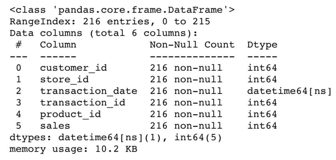
As you can see, our DataFrame includes 6 different columns, which are;
- customer_id
- store_id
- transaction_date
- transaction_id,
- product_id
- sales
The length of our features is 216. All features, except ransaction_date, have the same data type, int64. The transaction_date has a datetime64 data type.
Now, let’s continue with our second DataFrame, wfm_stores.
Let’s repeat the process and use the head() function to see the first rows.
wfm_stores.head()| store_id | store_brand | location |
|---|---|---|
| 1 | Clapham Junction | London |
| 2 | Camden | London |
| 3 | Fulham | London |
| 4 | Kensington | London |
| 5 | Piccadilly Circus | London |
Let’s use the info() function.
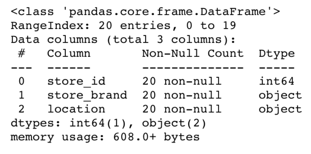
Okay, here we can see the wfm_stores DataFrame has 3 columns, which are
- store_id
- store_brand
- location
The length of our features is 20. The data types are int64 and object. You can see that store_id is the common column between our two DataFrames, which we will use to merge two DataFrames.
Now that we’ve finished the exploration step let’s start writing out the approach to solving the question.
2. Writing Out the Approach
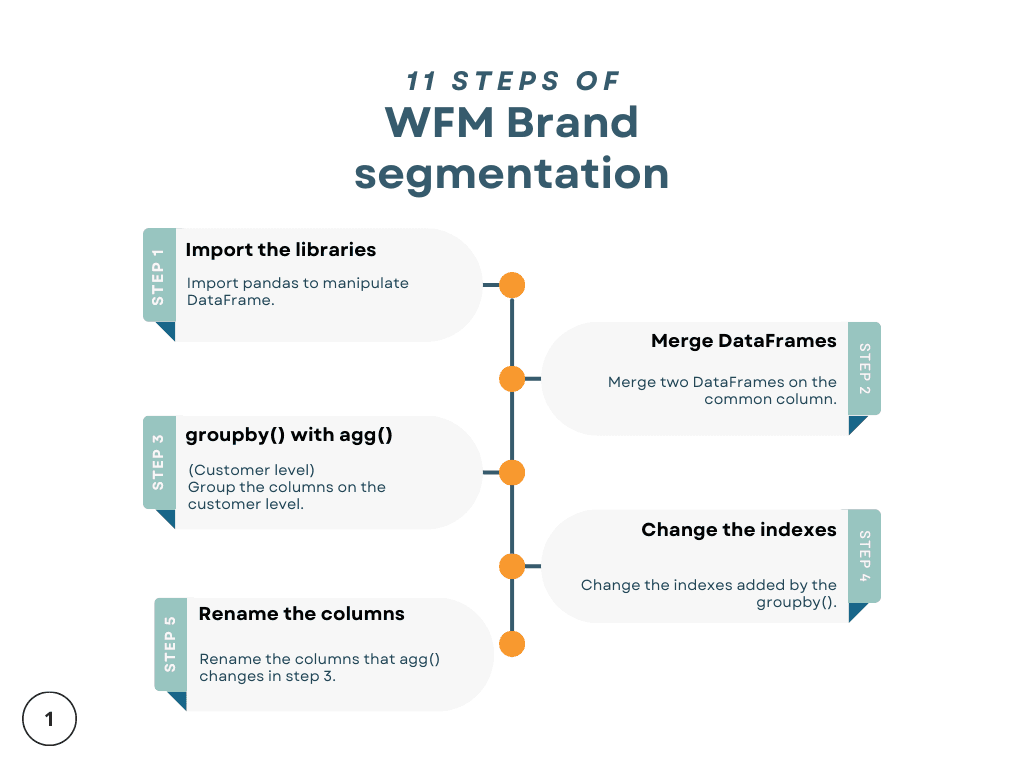
Let’s split this problem into codable stages. By doing that, we will not only frame the question but also speed up the solving process. Now, let’s split this problem into 11 steps, starting with importing the library, merging DataFrames, and finishing with final calculations to find the average basket size by brand and segment we defined according to the conditions.
Let’s start with importing the libraries.
Step 1: Import the Libraries
First, we will import pandas as pd to manipulate the data set.
Step 2: Merge DataFrames and Select the Variables.
Next, we will combine our DataFrames and then select the variables that will be needed in the further stages.
Step 3: The groupby() With the agg() Function.
Here, we will first select the year, then group the DataFrame by the customer and the store using groupby().
Then we will calculate the total sales by the transaction ID using the agg() function.
Step 4: Change the Index
In this step, we’ll change the indexes that the groupby() function adds in step 3.
Step 5: Change the Column Name
Now, we will rename the columns because the original name was replaced with the function name during calculations.
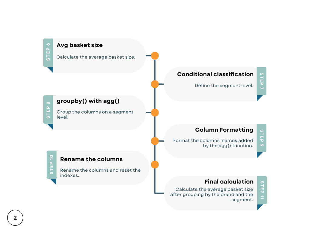
Step 6: Average Basket Size on a Customer Level
Here, we will calculate the average basket for each customer.
Step 7: Conditional Classification
We already calculated the basket size. With this step, we will create a three-segment column according to the threshold mentioned in the question. Here’s the reminder.
- If average basket size is more than $30, then Segment is “High”.
- If average basket size is between $20 and $30, then Segment is “Medium”.
- If average basket size is less than $20, then Segment is “Low”.
Step 8: The groupby() With the agg() Function on a Segment Level
Here, we will use the groupby() function with agg() function to calculate the total sales for each unique customer segmented by brand.
Step 9: Column Formatting
We will format the column names because after doing calculations and creating columns with the agg() function, the column names is not in the right format for us.
Step 10: Renaming Columns
We will rename the columns and reset the indexes that the groupby() function added two steps earlier.
Step 11: Final Calculation – Average Basket Size by Brand and Segment
Finally, we will calculate the average basket size after grouping by brand and segment.
3. Coding the Solution
Since we already split our problem into 11 different stages, we will now change this logic into code. When you are involved in complex coding questions, split the question into easy steps, and turn these steps into code, as we will do here. This will make your life (and coding!) much easier!
Step 1: Import the Libraries
First, import the pandas library as pd, which will be used for data manipulation throughout the rest of our article.
import pandas as pdStep 2: Merge DataFrames and Select the Variables.
We have two DataFrames, so to do further analysis, we should combine them. We will do this by using the merge() function and assigning the resulting DataFrame to the result variable.
We will merge this on the store_id column, a common column of both DataFrames.
result = pd.merge(wfm_stores, wfm_transactions, how='left', on='store_id')[['customer_id', 'store_brand', 'transaction_id', 'sales', 'transaction_date']]
Here is the output.
| customer_id | store_brand | transaction_id | sales | transaction_date |
|---|---|---|---|---|
| 1 | Clapham Junction | 1 | 13 | 2017-01-06 |
| 1 | Clapham Junction | 1 | 5 | 2017-01-06 |
| 1 | Clapham Junction | 1 | 1 | 2017-01-06 |
| 1 | Clapham Junction | 21 | 10 | 2017-01-01 |
| 15 | Clapham Junction | 109 | 70 | 2017-05-06 |
Step 3: The groupby() With the agg() Function
In this step, we will use the groupby() and agg() functions. Since we focused on these functions, let me explain these functions first, and then we will continue coding.
groupby()
The groupby() function allows us to split our DataFrame according to our needs. We can do this by using the by arguments inside it or group our DataFrame on more than one column. We will do exactly that in this step: add the columns to a list and use this list as an argument.
If you want to see more about the groupby() function, here is its official web page.
agg()
The agg() function will allow us to apply function or functions to the DataFrame or the DataFrame columns separately and creates a new column accordingly. We will do this by applying the nunique and sum functions to the transaction_id and the sales columns, respectively, to find the total sales for the unique transaction IDs.
If you want to see more arguments, here is the official library of the agg() function.
In the code below, we filter the results by including only rows with transaction dates in 2017 using the dt.year() function.
After that, we use the groupby() function to group the data by customer_id and store_brand. Then comes the agg() function to find the unique transaction_id (with the nunique function) and total sales (with the sum function).
result = result[result['transaction_date'].dt.year==2017].groupby(['customer_id', 'store_brand']).agg({'transaction_id':['nunique'],'sales':['sum']})
Here is the output.
| transaction_idnunique | salessum |
|---|---|
| 4 | 1640 |
| 5 | 920 |
| 1 | 100 |
| 1 | 866 |
| 3 | 910 |
Step 4: Changing the Index
Now, our result DataFrame has multi-level indexes, which we will remove by using the droplevel() function.
result.columns = result.columns.droplevel(0)
result
Here is the output.
| nunique | sum |
|---|---|
| 4 | 1640 |
| 5 | 920 |
| 1 | 100 |
| 1 | 866 |
| 3 | 910 |
Step 5: Changing the Column Name
Alright, now let’s change the column names using the rename() function. This will remove the indexes that group by added in step 3.
result = result.reset_index().rename(columns={'nunique':'transactions', 'sum':'sales'})
result
Here is the output.
| customer_id | store_brand | transactions | sales |
|---|---|---|---|
| 1 | 365 by WFM | 4 | 1640 |
| 1 | Clapham Junction | 5 | 920 |
| 1 | Fulham | 1 | 100 |
| 2 | 365 by WFM | 1 | 866 |
| 2 | Camden | 3 | 910 |
Step 6: Average Basket Size on a Customer Level
Here, we will calculate the average basket size for each customer by dividing the sales column by the transactions column and assigning the result to the avg_basket_size column.
result['avg_basket_size'] = result['sales']/result['transactions']
Again, to see the output add:
resultHere is the output.
| customer_id | store_brand | transactions | sales | avg_basket_size |
|---|---|---|---|---|
| 1 | 365 by WFM | 4 | 1640 | 410 |
| 1 | Clapham Junction | 5 | 920 | 184 |
| 1 | Fulham | 1 | 100 | 100 |
| 2 | 365 by WFM | 1 | 866 | 866 |
| 2 | Camden | 3 | 910 | 303.33 |
Step 7: Conditional Classification
We will classify the segments in this stage. First, we will define a custom function with lambda according to the conditions given to us. If avg_basket_size is greater than 30, the value will be assigned as ‘High’. If it is between 20 and 30, the value will be assigned as ‘Medium’; otherwise, it will be ‘Low.
result['segment'] = result['avg_basket_size'].apply(lambda x: (x > 30 and 'High') or (20 <= x <= 30 and 'Medium') or 'Low')
Here is the output.
| index | segment |
|---|---|
| 0 | High |
| 1 | High |
| 2 | High |
| 3 | High |
| 4 | High |
Step 8: Unique Customers With Total Sales – groupby() With agg() on Segment Level
Here we will group the results by store_brand and segment first. After that, we will usethe agg() function to find a unique customer ID by applying nunique() to customer_id. Then we will apply the sum() function to the transactions column to also find the total transaction.
result = result.groupby(['store_brand', 'segment']).agg({'customer_id':['nunique'],'transactions':['sum'], 'sales':['sum']})
Here is the output.
| customer_idnunique | transactionssum | salessum |
|---|---|---|
| 21 | 50 | 16883 |
| 2 | 3 | 44 |
| 9 | 17 | 4570 |
| 1 | 1 | 16 |
| 1 | 2 | 59 |
Step 9: Column Formatting
Take a look at the previous output. Especially pay attention to the column names.
Now, let’s see the change after we run the below code.
result.columns = result.columns.map('_'.join)
result
Let’s see the output to see the change.
| customer_id_nunique | transactions_sum | sales_sum |
|---|---|---|
| 21 | 50 | 16883 |
| 2 | 3 | 44 |
| 9 | 17 | 4570 |
| 1 | 1 | 16 |
| 1 | 2 | 59 |
Step 10. Renaming Columns
Here, we will change the column names after resetting indexes. Remember, we used to groupby() function in step 8, which changed indexes and names.
result = result.reset_index().rename(columns={'customer_id_nunique':'number_customers', 'transactions_sum':'total_transactions', 'sales_sum':'total_sales', 'store_brand':'brand'})Here is the output.
| brand | segment | number_customers | total_transactions | total_sales |
|---|---|---|---|---|
| 365 by WFM | High | 21 | 50 | 16883 |
| 365 by WFM | Low | 2 | 3 | 44 |
| Camden | High | 9 | 17 | 4570 |
| Camden | Low | 1 | 1 | 16 |
| Camden | Medium | 1 | 2 | 59 |
Step 11: Final Calculation – Average Basket Size by Brand and Segment
We’ve come to the last step where wher the final calculation awaits us. Remember that we have already done this calculation, but it was on a customer level. Now we are calculating this average basket size from the data set already grouped by brand and segmentation.
Remember, this is what the question asks.
“Summarize the number of unique customers, the total number of transactions, total sales, and average basket size, grouped by store brand and segment for 2017.”
Alright, now let’s calculate the average basket size.
result['avg_basket_size'] = result['total_sales']/result['total_transactions']
Adding this to previous steps, the complete code looks like shown below.
import pandas as pd

result = pd.merge(wfm_stores, wfm_transactions, how='left', on='store_id')[['customer_id', 'store_brand', 'transaction_id', 'sales', 'transaction_date']]
result = result[result['transaction_date'].dt.year==2017].groupby(['customer_id', 'store_brand']).agg({'transaction_id':['nunique'],'sales':['sum']})
result.columns = result.columns.droplevel(0)
result = result.reset_index().rename(columns={'nunique':'transactions', 'sum':'sales'})
result['avg_basket_size'] = result['sales']/result['transactions']
result['segment'] = result['avg_basket_size'].apply(lambda x: (x > 30 and 'High') or (20 <= x <= 30 and 'Medium') or 'Low')
result = result.groupby(['store_brand', 'segment']).agg({'customer_id':['nunique'],'transactions':['sum'], 'sales':['sum']})
result.columns = result.columns.map('_'.join)
result = result.reset_index().rename(columns={'customer_id_nunique':'number_customers', 'transactions_sum':'total_transactions', 'sales_sum':'total_sales', 'store_brand':'brand'})
result['avg_basket_size'] = result['total_sales']/result['total_transactions']
result- The dataset has already been loaded as a pandas.DataFrame.
- print() functions and the last line of code will be displayed in the output.
- In order for your solution to be accepted, your solution should be located on the last line of the editor and match the expected output data type listed in the question.
Here is the output you should get after running the code.
| brand | segment | number_customers | total_transactions | total_sales | avg_basket_size |
|---|---|---|---|---|---|
| 365 by WFM | High | 21 | 50 | 16883 | 337.66 |
| 365 by WFM | Low | 2 | 3 | 44 | 14.67 |
| Camden | High | 9 | 17 | 4570 | 268.82 |
| Camden | Low | 1 | 1 | 16 | 16 |
| Camden | Medium | 1 | 2 | 59 | 29.5 |
| Clapham Junction | High | 19 | 41 | 8823 | 215.2 |
| Clapham Junction | Low | 1 | 1 | 10 | 10 |
| Fulham | High | 14 | 24 | 6667 | 277.79 |
| Fulham | Low | 1 | 1 | 15 | 15 |
| Kensington | High | 5 | 7 | 1900 | 271.43 |
| Kensington | Low | 1 | 1 | 12 | 12 |
| Kensington | Medium | 1 | 1 | 20 | 20 |
| Piccadilly Circus | High | 2 | 2 | 638 | 319 |
| Piccadilly Circus | Medium | 1 | 2 | 41 | 20.5 |
| Richmond | High | 3 | 4 | 2620 | 655 |
| Stoke Newington | High | 2 | 3 | 973 | 324.33 |
| Whole Foods Market Daily Shop | High | 12 | 26 | 7776 | 299.08 |
| Whole Foods Market Daily Shop | Low | 1 | 2 | 14 | 7 |
Conclusion
In this blog post, we have successfully solved the Whole Food Market interview question using the agg() and groupby() functions in Python.
We first explored the dataset, outlined our approach, and then walked through the coding process. By the end, we calculated the average basket size for each customer and segmented them into different groups based on their activity.
If you want to improve your Python coding skills and prepare for future interviews, do not forget to check out our platform, which includes a wide range of Python coding questions, data projects from companies like Forbes, Meta, Google, Whole Food Market, and more.
Share