Today’s article discusses the workings of content-based filtering systems. Learn about it, what its algorithm does, and how to build it in Python.

Nowadays, the recommendation system can be viewed as one of the most successful machine learning applications in real-world business problems.

If you consume any form of social media, such as YouTube, Instagram, Twitter, Facebook, etc., then chances are that you’ve already got some exposure to recommendation systems. Let’s take YouTube as an example. Once you watch several videos related to photography, then you’ll notice that there are more and more photography videos appearing on your main landing page.

Netflix is also a company that uses a recommendation system in its everyday operation. Once you watch several movies about detectives solving murder mysteries, then you’ll notice that more and more movies with crime and thriller genres are being recommended to you. A recommendation system is designed to make you spend more time on a certain platform or to make you buy certain products.

In practice, there are at least three different types of recommendation systems: content-based filtering, collaborative filtering, and context-aware filtering. In this article, we’re going to focus solely on the first algorithm, which is content-based filtering. Specifically, we’re going to learn what content-based filtering actually is and how to build a content-based recommendation system with Python.

So let’s start with some introduction to content-based recommendations!

What is Content-Based Filtering?

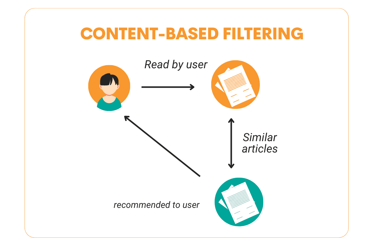
Content-based filtering is a type of recommendation system that is able to give each user a very personalized item recommendation. If you like to watch Marvel movies, then you’ll most likely watch Batman in the future compared to The Fault in Our Stars. This is what content-based filtering tries to tackle. This algorithm gives you item recommendations based on the item that you have liked in the past.

The one thing that really distinguishes the content-based recommendation system from other recommendation systems is that it doesn’t really need other people’s data. All of the recommendations are made based on just your data and your preference.

So now you might ask: how does a content-based recommendation algorithm work such that it can recommend similar items?

There are a lot of different ways how content-based filtering can be done, i.e., it can recommend items based on one or several features. As an example, let’s say that you liked The Dark Knight in the past. Content-based filtering will then recommend movies that are similar to The Dark Knight in one or several features, which could be the genre, the movie summary, the movie director, etc.

Another important thing to note is that this recommendation system uses similarity algorithms to recommend similar items to the ones that you have liked in the past. Among several similarity algorithms, cosine similarity is the most common algorithm to use. In a nutshell, cosine similarity measures the distance between two vectors in the high dimensional space with the following formula:

where x is the embedding vector of the item that you have liked in the past, and y is the embedding vector of another item. (x.y) term indicates the dot product between two vectors, while (||x||*||y||) term indicates the cross product between two vectors.

If we use cosine similarity, then we will get a value within the range of -1 to 1. The closer the value to 1, the more similar the items will be. Meanwhile, the closer the value to -1, the more dissimilar the two items will be.

Content-Based Filtering: Important Terms

Before we take a look at an example of how content-based filtering is implemented in real-life, we need to know first about several important terms that usually appear whenever we learn about this recommendation system.

User Matrix

User matrix refers to a 2-dimensional matrix that represents all the information regarding the users. This could be the data regarding your customers or subscribers, for example. Each row of the matrix normally represents one specific user, whilst the column represents the numerical representation of each user. We will talk about this numerical representation soon in this section.

Item Matrix

The concept of the item matrix is the same as the user matrix. It consists of a 2-dimensional matrix that represents all of the information regarding the items. This could be a movie, an electronic device, or literally any product that you offer to the users. Each row of the item matrix represents one specific item, whilst the column represents the numerical representation of each item.

Features

The numerical representations of each user and item (which occupy the columns of the user matrix and item matrix) can also be called features. As computers can only process numeric data, the generation of these features is a very crucial step to make sure that high-quality recommendations can be produced.

As an example, the features of a specific movie can be its synopsis. However, the information regarding synopsis only comes in the form of text, and computers can’t process information in the form of text. Thus, what we normally do is convert the text into its numerical representation with different kinds of methods, such as TF-IDF or count vectorizer. We will learn how to convert our features into their numerical representation later in this article.

User-Item Matrix

As the name suggests, a user-item matrix is the combination of a user matrix and an item matrix. User-item matrix is particularly important in recommendation system algorithms as the final step before the recommendations are given to each user. In a nutshell, a user-item matrix contains the preference of each user with respect to each item after a matrix factorization process that can be done via several methods.

In the step-by-step example of content-based filtering later on in this article, we will see how this user-item matrix can be obtained from a user matrix and an item matrix.

Recommendation Generation in Content-Based Filtering

In the previous section, we know that there are two essential matrices that we need to have to generate item recommendations with content-based filtering: a user matrix and an item matrix. A user matrix is basically a matrix that stores the information regarding each user, and likewise, an item matrix is a matrix that stores the information regarding the items that we want to sell.

The question that we will answer in this section is: how does content-based filtering generate recommendations based on those matrices?

There are a few methods to do so, such as dot product similarity, pairwise distance, and cosine similarity. We will talk about each of them, and let’s start with dot product similarity.

Dot Product Similarity

Dot product similarity is very useful for finding the similarity between two numerical representations of things. To illustrate how dot product similarity works, let’s imagine we have a tiny item matrix, which consists of four movies, and each movie has 2-dimensional features. Here’s what our item matrix looks like:

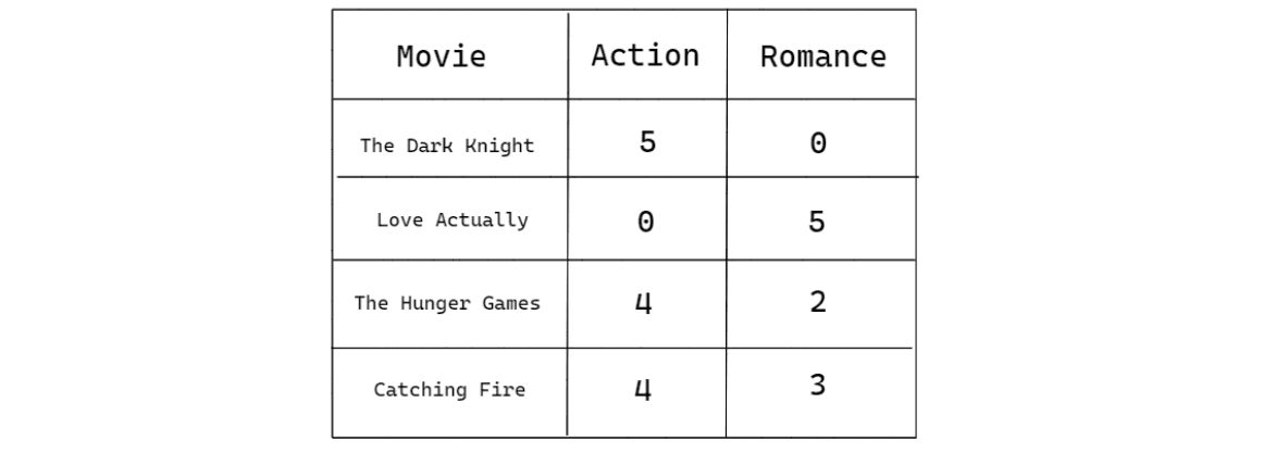
From the table above, how do we capture the similarity between a pair of the movies above? If we use our intuition, we know there is nothing in common between The Dark Knight and Love Actually, as the former is an action movie, while the latter is a pure romance movie. Meanwhile, we would know that The Hunger Games is similar to Catching Fire, as Catching Fire is basically the sequel to The Hunger Games.

Capturing the similarity of items with dot product similarity is simple. All you have to do is to multiply each element of the features between a pair of movies. Let’s say that we want to know the similarity between The Dark Knight and Love Actually, as well as between The Hunger Games and Catching Fire, we can do so by doing the following:

The multiplication operation that we just did above is also called the dot product operation. The result of the dot product also makes sense and confirms our intuition that the similarity between The Hunger Games and Catching fire should be higher than between The Dark Knight and Love Actually.

Pairwise Distance

Aside from using the dot product of each item’s features, we can also measure the similarity with the pairwise distance. The intuition behind pairwise distance is straightforward. When two items are placed close to each other in vector space, then the distance between them is small, hence the higher the similarity. Vice versa, the further two items are placed in the vector space between one another, the higher the distance, hence the lower the similarity.

We can use the example from dot product similarity above to make things clearer. Each movie has 2-dimensional features. Since it’s just 2D, then we can actually draw their place in the vector space as follows:

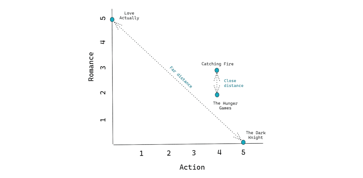
As you can see from the graph above, the x-axis represents the action genre, whilst the y-axis represents the romance genre. From the visualization above, we can notice that The Dark Knight and Love Actually are placed far away from each other. Meanwhile, The Hunger Games are placed close to each other.

To compute the distance between two items in the vector space, what we can do is draw the shortest line that connects the two items, and the length of that shortest line is normally called the Euclidean distance, as visualized by the dotted lines in the visualization above.

Cosine Similarity

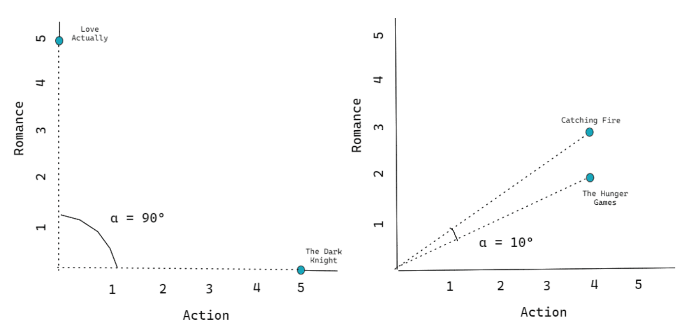
Another method to compute the similarity between two items is by looking at their angle in the vector space. Take a look at the visualization of the vector space above as an example. If we measure the angle between any pair of movies with respect to the origin coordinate (0,0), then we can see that if two movies are placed close to each other, then the angle will be small. Likewise, if two movies are placed far apart, then the angle will be large, as you can see in the visualization below:

However, measuring the similarity by the angle itself is not quite intuitive. We need a helper function that can map the angle formed by any pair of items in a vector space into a value that has a range between -1 to 1. And this is where the cosine function comes in.

If you take a look at the visualization on the left-hand side, the angle formed between The Dark Knight and Love Actually is exactly 90 degrees. On the right-hand side, let’s say the angle formed between The Hunger Games and Catching Fire is 10 degrees. With the cosine function, we get the following final value:

As you can see, the cosine function helps to transform our similarity score in a much more intuitive way. The closer the cosine similarity to 1, the more similar the two items are.

Example of Content-Based Filtering

So far, we have learned about the theory of content-based filterings. In this section, we’re going to see an example of how it actually works. The example will revolve around movies and how content-based filtering recommends items based on the movie’s genres.

Suppose you’re subscribing to Netflix, and there are only six movies on that platform: Batman Begins, The Dark Knight, Twilight, Toy Story, Love Actually, and Up. Out of these six movies, you’ve seen three of them, and you give each of them a rating score that ranges between 1 to 10, with 1 being the worst and 10 being the best. Let’s say that these are the rating that you gave to each of the movies that you’ve seen:

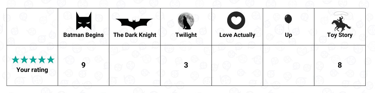
And this is what a user matrix looks like. It contains specific information about you and other people as users. In this case, the user feature would be the rating that you give to each movie. It’s important to note that in this specific example, we only consider you as the only user such that it also can be called a user vector instead of a user matrix.

Now the question is: how does a content-based algorithm recommend another movie given the user matrix above?

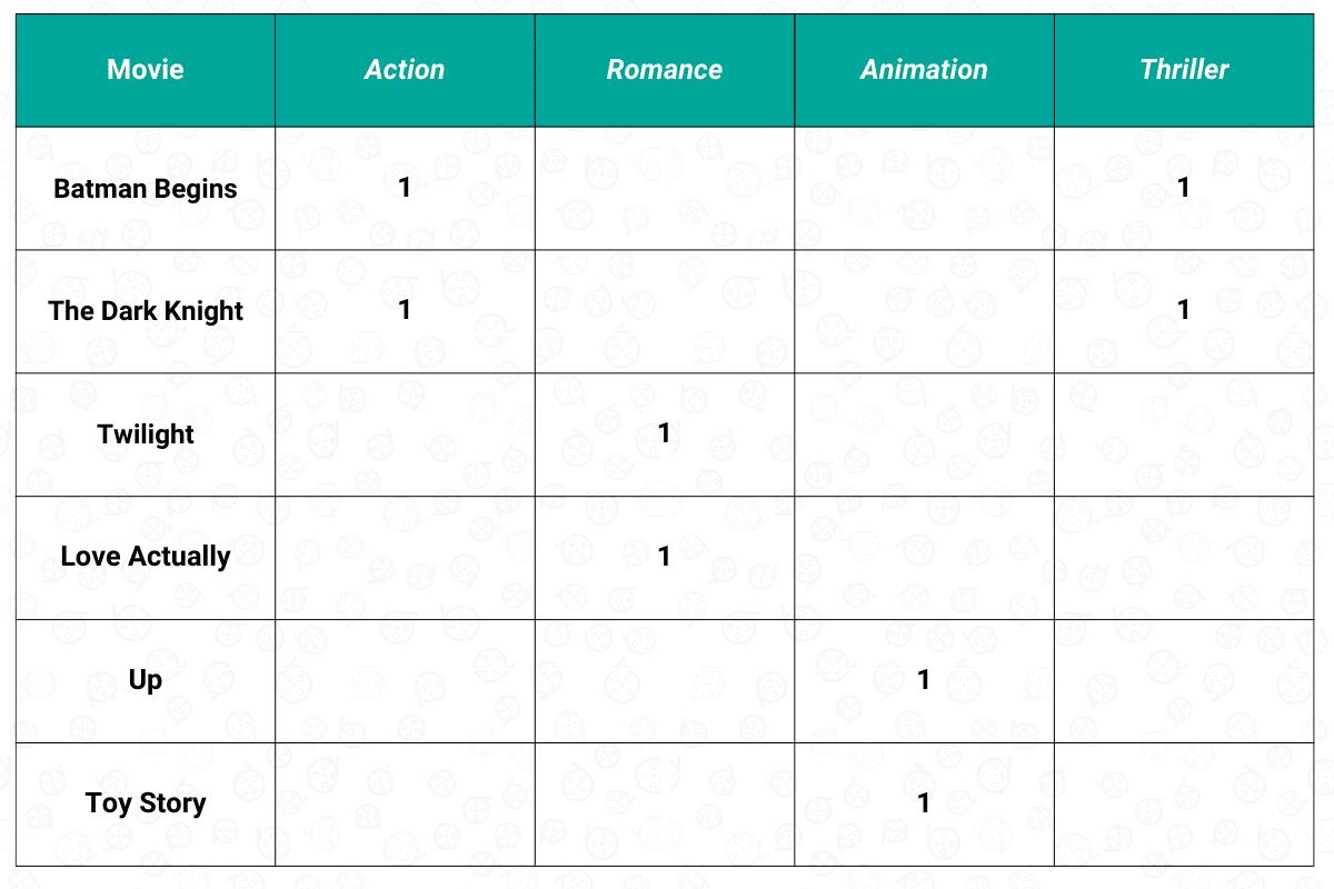
To answer the question above, we need to look at our second matrix, which is the item matrix. As you might already know, our item would be the movie. Each movie has a genre, and the genre of each movie will act as the feature. The genre of a movie is normally binary encoded, i.e., the value will be 1 if a movie has that specific genre and 0 otherwise. In our example of six different movies above, the item matrix would look something like this:

After this step, we now have two different matrices: the user matrix and the item matrix. The next step would be computing the weighted item matrix based on the movie rating that we have in the user matrix, as you can see below:

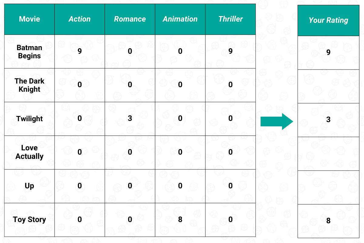
The weighted item matrix above can also be called the user-item matrix. It can be obtained by using the dot product between the user matrix and the item matrix that we have before. If you take a look at the example above, we gave Batman Begins a 9 out of 10 rating, and we know that it has a genre of Action and Thriller. Thus, we multiply 9 by 1 in each of these genres, and we do the same step for each movie that we have rated before, i.e., Twilight and Toy Story.

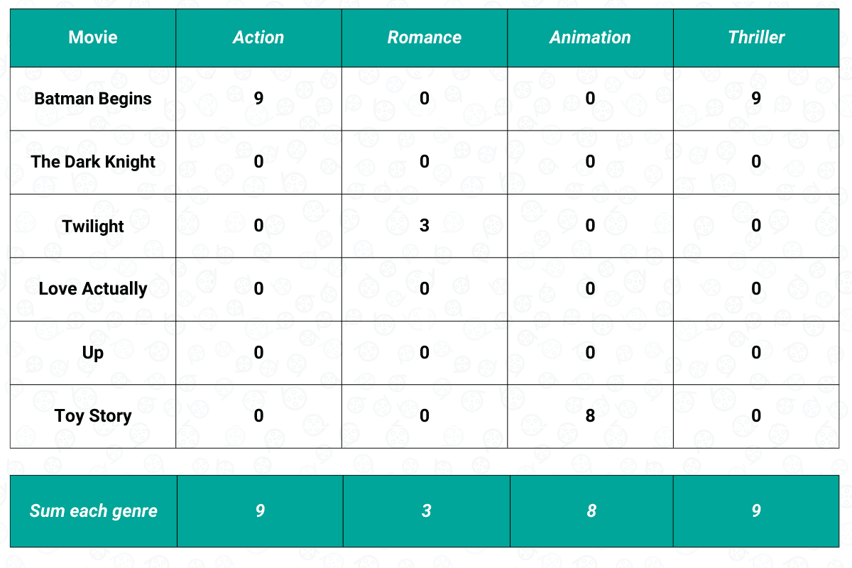
Once we have the user-item matrix, we need to sum the weighted score of each feature, as you can see below:

Now that we have the sum of the weighted score of each feature, then we need to normalize the score such that when we sum all of the features, the score adds up to one. After the normalization process, this is what our final user-item matrix will look like:

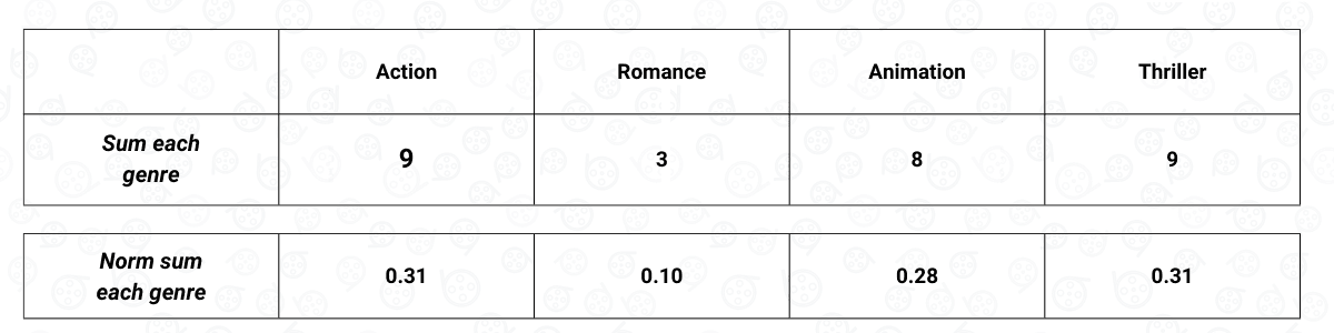
The final normalized user-item matrix above shows us our preference with respect to the feature of a movie, which in our case, is the movie genre. Based on the normalized user-item matrix above, we can see that we have a high preference for a movie that has an Action and a Thriller genre. On the other hand, it is very likely that we won’t like a movie that has a Romance genre.

To make recommendations of items, content-based filtering will then once again use the dot product between the normalized user-item matrix above with the user vector. As an example, The Dark Knight has a genre of Action and Thriller. From the normalized feature that we have calculated above, we know that ‘Action’ has a value of 0.31, while ‘Thriller’ also has a value of 0.31. The dot product between these values and the value in the user feature vector will then be calculated. As a result, we have 0.62 for The Dark Knight.

We do the same step for every movie that we haven’t watched yet, and this is what the final result looks like:

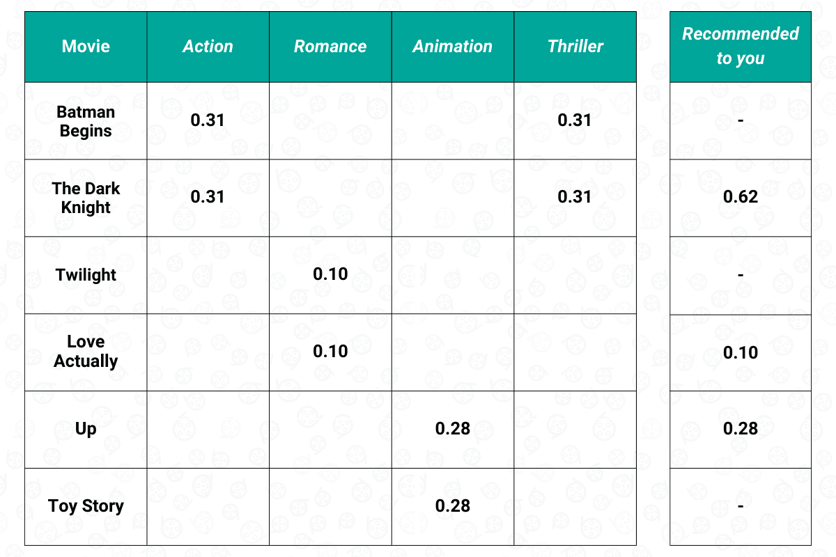
The final result above can be viewed as our preference. Thus, the content-based filtering will then recommend The Dark Knight, followed by Up and Love Actually.

As you can see from the step-by-step of how content-based filtering works above, we don’t need the data of other people. All of the recommendations are based on your preference and will be somewhat similar to the things that we have liked in the past.

Now that we know how content-based filtering actually works let’s get straight into the implementation.

Content-Based Filtering Implementation

In this section, we’re going to implement a content-based filtering algorithm with the help of Python. The data that we’re going to use is the Movielens dataset, which is a dataset that’s quite popular to test out a recommendation system. The dataset contains 45,000 movies, each with its own metadata such as genre, runtime, cast, keyword, etc. If you want to follow along, you can find and download the code on this Kaggle page.

As mentioned in the previous sections, there are a lot of ways to build a content-based recommendation system in the sense that we can choose which feature we want the recommendation based on.

In the implementation below, we’re going to build a movie recommendation system with content-based filtering. Specifically, we’re going to build a recommendation system based on the movie's summary, and thus, we only need one file from the dataset, which is movies_metadata.csv . Let’s first start importing all of the necessary libraries for this project as well as loading the data.

import pandas as pd
from sklearn.feature_extraction.text import TfidfVectorizer
from sklearn.metrics.pairwise import cosine_similarity

# Read the data
movie_data = pd.read_csv('movies_metadata.csv')

Now that we load all of the data, we need to create three different variables: one for the movie title, one for the movie summary, and another as a mapping between the movie title and indexes.

# Movie summary data, fill null value with empty string
movie_summary = movie_data['overview'].fillna('')

# Movie title data
movie_title_data = movie_data['original_title']

# Map movie title to its index
movie_to_index = pd.Series(movie_data.index, index=movie_data['title']).drop_duplicates()

The variable movie_summary above will be our key feature to determine which movie that we should recommend to a specific user. If a user liked Furious 7 in the past, then we want to recommend a movie that has a similar summary to Furious 7.

To do that, we need to process the movie summary of each movie such that the computer can make use of it. As you might already know, computers can’t process information in the form of text. Thus, we need to convert all of the texts in the movie_summary variable into its numerical representation, and to do this, we can use a method called TF-IDF.

TF-IDF stands for Term Frequency-Inverse Document Frequency. This method is very beneficial in the area of text analysis as it measures the relevancy of each word of a document in a collection of documents. This means that if a certain word appears very frequently in a collection of documents, then the TF-IDF score of that word will be low. The TF-IDF score measures the importance of a word in a document.

This concept makes sense because we can expect that words like ‘if’ and ‘and’ will appear a lot in each of the documents. Thus, we need to put those words in a low rank as those words have low importance to a document. Meanwhile, if the word ‘car’ appears a lot in one document but not in the other documents, then we can say that the word ‘car’ is very important to that particular document. Thus, this word will rank high in the TF-IDF score.

TF-IDF can be computed with the following formula:

where:

tf_x,y: the frequency of term x within document y
N: total number of documents
df_x: total number of documents which contain term x

As the result of the equation above, if a word is used very frequently in many documents, then its value will approach 0. Otherwise, the TF-IDF score will approach 1.

TF-IDF algorithm can be easily applied in Python with the help of the scikit-learn library by using TfidfVectorizer class, as you can see in the code snippet below:

tfidf = TfidfVectorizer(stop_words='english')
movie_matrix= tfidf.fit_transform(movie_summary)

The stop_words argument there is beneficial to remove the English stop words such as ‘the’, ‘a’, ‘an’, etc., as we know that those words appear a lot in each of the documents. The next thing that we should do is to train our TF-IDF model on the whole entirety of the data, which in our case is the movie summary. What we get as the training result is a user-feature matrix that you’ve learned from the previous section. Let’s find out the shape of this matrix.

movie_matrix.shape
>>> (45466, 75827)

As you can see, the matrix has a shape of (45466, 75827), meaning that we have 45466 rows and 75827 columns. The rows represent the item, which in our case is the movie title, and the columns represent the feature, which in our case are the words available in our entire movie summary data.

With this movie_matrix, now each movie is represented by a vector of size 75827. We can use this matrix to calculate the similarity between each movie. As mentioned in the beginning, there are a few metrics commonly used to calculate the similarity in real life. However, the most commonly used one is cosine similarity, and this is what we’re going to implement in this example.

Now let’s generate some movie recommendations based on the movie matrix that we have so far. Suppose we liked Furious 7 in the past, and we want movie recommendations that are similar to that. The first thing to do would be fetching the index of Furious 7 movie with the movie_to_index variable. Next, we can use the corresponding index to fetch its summary, as you can see in the code snippet below:

movie_title = 'Furious 7'

# Get the index of movie title
idx = movie_to_index[movie_title]

# Get the corresponding movie summary
movie_test_summary = [movie_summary[idx]]

The next thing that we should do is transform the movie summary of Furious 7 into its numerical representation with TF-IDF method. Since we have trained our TF-IDF model before, then we should use the transform method instead of fit_transform, as you can see below:

# Fetch the TF-IDF vector of the corresponding movie
movie_test_matrix = tfidf.transform(movie_test_summary)
print(movie_test_matrix.shape)
>>> (1, 75827)

After the transformation, you now get basically a vector of size 75827. This is the numerical representation of Furious 7. Next, we can compare its similarity with each of the movies in the movie matrix that we have created before.

# Calculate the cosine similarity between the movie and each of the entry in   # movie_matrix

sim_scores = cosine_similarity(movie_test_matrix, movie_matrix).tolist()[0]
print(len(sim_scores))
>>> (45466)

The similarity scores that you get will have a length of 45466, which is equal to the total number of movies in our movie matrix. This means that the sim_scores variable contains the similarity between Furious 7 and each movie in our movie matrix. Now what we need to do is to sort the similarity scores from the highest to lowest score and then fetch the 10 movies with the highest similarity score.

sim_scores = sorted(enumerate(sim_scores), key=lambda i: i[1], reverse=True)


# Fetch the top 10 recommended movies
sim_scores = sim_scores[1:11]

The final thing that we need to do next is to fetch the recommended movies’ indexes, and then map the indexes back to their corresponding movie title, as you can see below:

# Fetch the recommended movies' indexes
movie_indexes = [i[0] for i in sim_scores]

# Print the title of recommended movies
 print([movie_title_data[i] for i in movie_indexes])

>>> ['The Fast and the Furious',
 'Fast & Furious 6',
 'Los violadores',
 'Fast Five',
 'Genius on Hold',
 'Youth Without Youth',
 'The Skydivers',
 'Aenigma',
 'The Cell',
 'Urban Justice']

As you can see, as we liked Furious 7 in the past, our content-based recommender system will recommend similar movies to us such as The Fast and The Furious, Fast Five, Fast & Furious 6, etc.

To make everything cleaner, we can encapsulate all of the steps that we have done above into a single function such that when we want a movie recommendation, all we need to do is to provide the movie title.

def get_recommendation(movie_title, movie_matrix=movie_matrix):

  # Get the index of movie title
  idx = movie_to_indexes[movie_title]

  # Get the corresponding movie summary
  movie_test_summary = [movie_summary[idx]]

  # Fetch the TF-IDF vector of the corresponding movie
  movie_test_matrix = tfidf.transform(movie_test_summary)

  # Calculate the cosine similarity between the movie and each of the entry in                                 #   movie_matrix

  sim_scores = cosine_similarity(movie_test_matrix, movie_matrix).tolist()[0]
  sim_scores = sorted(enumerate(sim_scores), key=lambda i: i[1], reverse=True)

  # Fetch the top 10 recommended movies
  sim_scores = sim_scores[1:11]

  # Fetch the recommended movies' indexes
  movie_indexes = [i[0] for i in sim_scores]

  # Return the title of recommended movies
  return [movie_title_data[i] for i in movie_indexes]

Now when we want a movie recommendation, we need only to call the function above and provide the movie title as the argument.

get_recommendation('Toy Story')

>>> ['Toy Story 3',
 'Toy Story 2',
 'The 40 Year Old Virgin',
 'Small Fry',
 "Andy Hardy's Blonde Trouble",
 'Hot Splash',
 'Andy Kaufman Plays Carnegie Hall',
 'Superstar: The Life and Times of Andy Warhol',
 'Andy Peters: Exclamation Mark Question Point',
 'The Champ']

In the example above, we use the movie summary as the only feature for our content-based movie recommendation system. However, you can be creative and use the combination of other features provided by the dataset such as the keyword, genres, director, etc.

The Pros and Cons of Content-Based Filtering

Like any other type of recommendation system, content-based filtering has its own pros and cons. Whether or not you should apply this recommendation system totally depends on your use case and the data that you have.

Pros

Let’s talk about the advantages of using content-based filtering:

1. It Doesn’t Need Data from Other Users

The main biggest pro of content-based filtering is the fact that we don’t need other users’ data to recommend items to a particular user. Once we have inputs from a particular user, then we can straight away give a recommendation to that user. Thus, content-based filtering would be ideal to be used in a company where the pool of users is not that big or in a company that has a big pool of users but not a lot of interactions or inputs made by each user.

2. High-Quality Recommendation

The fact that content-based filtering doesn't need data from other users also means that the quality of the recommendation will be highly personalized to each user’s preference. If you like The Avengers, content-based filtering will recommend similar movies like Iron Man or Captain America instead of Twilight to you. Meanwhile, if we use collaborative filtering, there is a chance that we will get a movie recommendation that’s not quite similar to The Avengers. Thus, content-based filtering would also be ideal for a company that sells a single item with several features, for example, movies, laptops, phones, headphones, etc.

3. Avoid cold start problem

In comparison with collaborative filtering, content-based filtering gives better results when there are only a few entries in the database. As an example, let’s say that you have a new platform, and there are only a few inputs from users. Content-based filtering can give each user better early recommendations as it only needs each user’s preference, whilst collaborative filtering needs data from several users. Once you grow your platform and there are more and more inputs from users, then collaborative filtering can be used instead of content-based filtering.

4. Easy to Implement

As it only needs the data from each user, then the implementation of content-based filtering in terms of data science and programming perspective is much simpler than the other recommender systems like collaborative filtering. One of the challenges of applying content-based filtering is choosing the combination of features to give each user high-quality recommendations.

Cons

However, content-based filtering is not by any means a free lunch, meaning that there are also downsides to it. Here are some of the disadvantages of using content-based filtering, such as:

1. Lack of Diversity

The main disadvantage of using content-based filtering is the lack of diversification in terms of the recommendation that you’re getting. As an example, let’s say that you liked Toy Story in the past. With content-based filtering, you’ll get recommendations that are similar to Toy Story, such as Toy Story 2, 3, 4, Up, Wall-E, etc., but you’ll never get recommendations of great movies from another genre. This means that you’re forced to always be inside of your bubbles without having a chance to explore another great movie that might have different features from the movie that you liked.

2. Scalability and Consistency Issue

The next disadvantage of content-based filtering is the fact that it’s difficult to scale, especially as the number of your data entry grows exponentially. This is because every time you have a new product or item, you need to add its attribute. Imagine if you have a lot of new products, then the task of defining the attribute of these products would be time-consuming, thus not really scalable.

The fact that the features of a new product need to be hand-engineered also raises another concern, which is a consistency issue. If there is more than one person that assigns the attributes of a new product, there might be different interpretations between one person or another of how the features should be assigned. Thus, content-based filtering requires subject matter experts to ensure the consistency and the right handling of the features of a new product.

Conclusion

In this article, we have learned everything that we need to know about content-based filterings, such as what it actually is, how it is implemented in theory and code, as well as its pros and cons.

Content-based filtering is a great recommendation system to use, especially when you have a platform with only a few inputs from the user. This recommendation system allows you to give a user high-quality recommendations just by looking at one particular item that the user has liked in the past. However, the lack of variation in the recommendations is still the main drawback of content-based filtering, which can be tackled if you use other recommendation systems, such as collaborative filtering.

Now that you learned about the content-based recommendation, you can apply your knowledge to answer some of the non-coding challenges available on StrataScratch:

• How to build a recommendation system
• Restaurant recommendation
• Replacement recommendation