PCA Analysis in Python for Beginners

A Practical Walkthrough of Principal Component Analysis with Real-World Examples in Python

One of the most common methods for reducing the number of features in machine learning is Principal Component Analysis (PCA). But why do you need to reduce them? Because it helps you find the most important ones and ignore the rest. This cuts down the computational cost and speeds up your model.

For example, in image recognition, you can compress hundreds of pixel features into a handful of principal components while still capturing most of the important variation. Similarly, in finance, you can reduce dozens of correlated market indicators into a few composite risk factors that explain most of the movement.

In this article, we’ll discover how to use PCA in Python step by step, including the logic, math, and a real project.

PCA Analysis Python: What It Is and Why It Matters

Let’s say you are trying to predict house prices and you have 10 columns, like square footage, number of rooms, distance from the city, and so on.

Some of these columns may be giving you the same kind of information. PCA finds patterns in these columns and builds new axes to represent the data more efficiently.

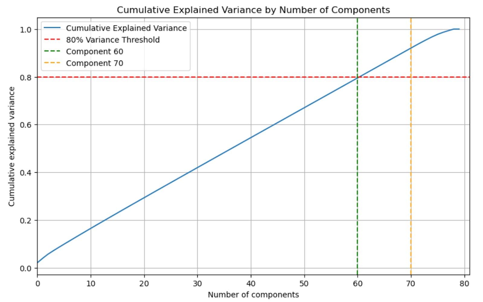
These new axes are called principal components. Each one shows how much of the total variation in the data it can explain. For example, in the graph below, you need between 6 components to explain 80% of the data.

When to Use PCA Analysis in Python

You don’t always need PCA. But in some cases, for instance, if your dataset is too large and your computational power is limited, it can really help.

It reduces the number of columns while keeping most of the critical signals. It’s also useful when some columns are highly correlated. PCA combines them into fewer, uncorrelated components.

Another reason to use PCA is for visualization. It helps you project high-dimensional data into 2D or 3D to spot clusters or outliers. But if your dataset is already small and clean, PCA might not help. Sometimes it can even remove signals that your model actually needs.

If you’re familiar with PCA in other languages or want to compare how it’s done elsewhere, you can see how it's implemented in principal component analysis in R for another perspective.

Math Behind PCA in Python

PCA works in a few simple steps.

• First, it centers your data by taking away the mean of each column.
• Then it checks how the columns vary together.
• Based on that, it finds new directions that capture the most variation in the data.

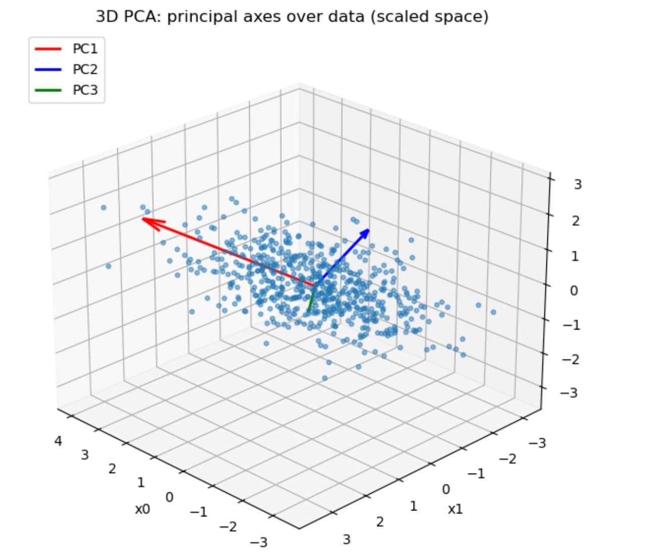
These directions are ranked by how much information they hold. You can then choose how many to keep, depending on how much variance you want to explain.

You can see these new directions in the plot below; the red, blue, and green arrows show how PCA finds the first three principal components, each capturing a different amount of variation in the data.

Setting Up Your Python Environment for PCA Analysis

To run PCA in Python, you only need a few basic packages. Here is the code to install the packages:

pip install pandas numpy matplotlib scikit-learn

Once you have installed them, here is the code to load them.

import pandas as pd
import numpy as np
import matplotlib.pyplot as plt
from sklearn.preprocessing import StandardScaler
from sklearn.decomposition import PCA

In the next section, we’ll load a real dataset and walk through each PCA step with code.

Real-World PCA Analysis in Python: DoorDash Delivery Duration Case Study

This is a real data science take-home assignment in the recruitment process for data science positions at DoorDash. The goal is to predict the total duration of the delivery process by examining order details, market activity, and estimated times. Here is the link to this data project.

Loading and Preparing Data for PCA Analysis in Python

Let’s load the data and take a quick look at it.

import pandas as pd

df = pd.read_csv("historical_data.csv")
df.head()

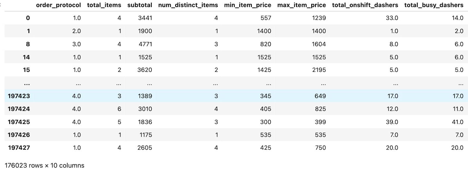
Here are the first few rows of the data.

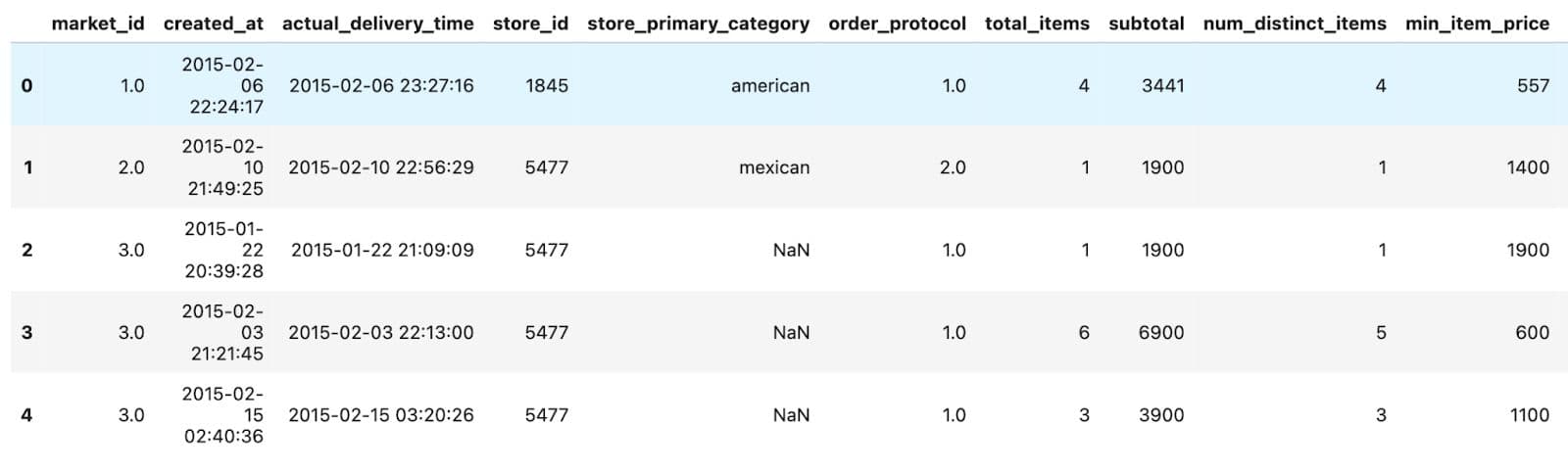
In the first few rows, we can see order timestamps, basic store details, item counts, and pricing information per order. Now let’s check all of the columns.

df.info()

Here is the output.

The full dataset includes columns related to store and order details, market activity at the time of order, internal delivery estimates, and all the timestamps needed to compute total delivery time.

Data Preprocessing

Before applying PCA, we performed a few basic preprocessing steps to prepare the dataset. One of the first things we needed was a column for delivery duration, but this wasn’t directly provided. We had to calculate it using two timestamp columns: `created_at` and `actual_delivery_time`.

Here’s how they looked at first:

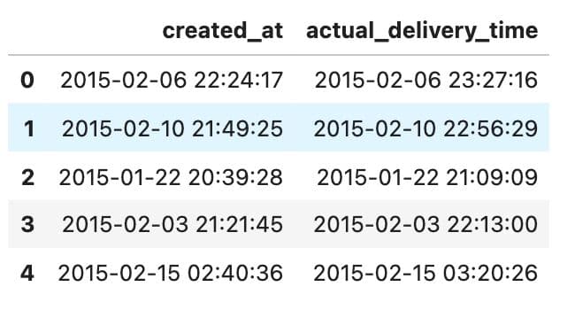
We converted them into `datetime` format and created a new column with the delivery duration in seconds. This will be our target variable for modeling.

Since PCA is an unsupervised feature reduction method, we will later drop this target column before running PCA.

df["created_at"] = pd.to_datetime(df["created_at"])
df["actual_delivery_time"] = pd.to_datetime(df["actual_delivery_time"])

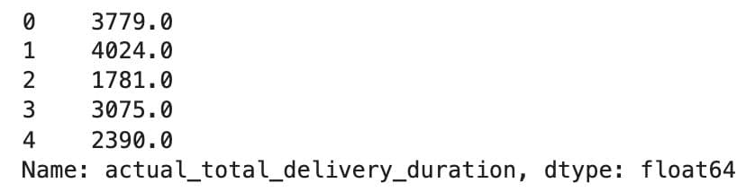
df["actual_total_delivery_duration"] = (
    df["actual_delivery_time"] - df["created_at"]
).dt.total_seconds()

df["actual_total_delivery_duration"].head()

Here is the output.

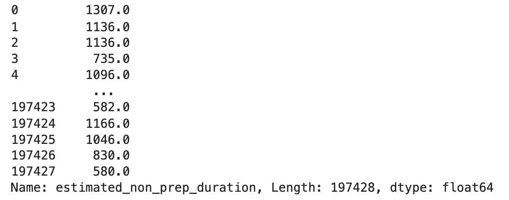
Next, we engineered a new feature called `estimated_non_prep_duration`, which combines the estimated driving time and order placement time:

df["estimated_non_prep_duration"] = (
    df["estimated_store_to_consumer_driving_duration"] +
    df["estimated_order_place_duration"]
)
df["estimated_non_prep_duration"]

Here is the output.

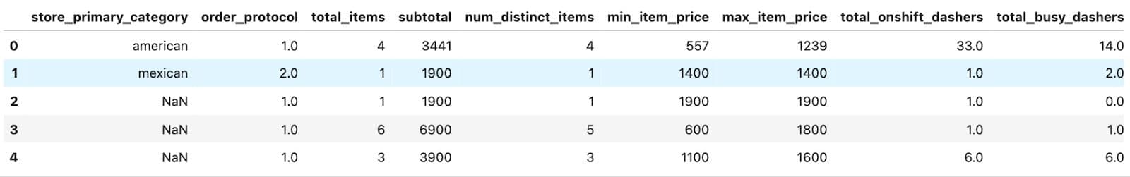
We’ll also remove the columns that don’t provide meaningful patterns for PCA, such as IDs, raw timestamps, and the original duration values:

drop_cols = [
    "store_id", "market_id",
    "estimated_order_place_duration", "estimated_store_to_consumer_driving_duration",
    "actual_total_delivery_duration", "created_at", "actual_delivery_time"
]

df = df.drop(columns=drop_cols, errors="ignore")
df.head()

Here is the output.

Next, we’ll clean missing values and select only numerical columns:

df_clean = df.dropna()
numeric_cols = df_clean.select_dtypes(include=["float64", "int64"]).columns
X = df_clean[numeric_cols]
X

Here is the output.

Applying PCA Analysis in Python Step by Step

Finally, we’ll scale the data to make it suitable for PCA and then check how much variance each component explains. Here is the code.

from sklearn.preprocessing import StandardScaler
from sklearn.decomposition import PCA
import matplotlib.pyplot as plt

scaler = StandardScaler()
X_scaled = scaler.fit_transform(X)

pca = PCA()
pca.fit(X_scaled)

cumulative_variance = pca.explained_variance_ratio_.cumsum()

plt.figure(figsize=(8, 5))
plt.plot(range(1, len(cumulative_variance) + 1), cumulative_variance, marker='o')
plt.axhline(y=0.95, color='r', linestyle='--', label='95% Variance Threshold')
plt.title('Cumulative Explained Variance by Number of Components')
plt.xlabel('Number of Components')
plt.ylabel('Cumulative Explained Variance')
plt.grid(True)
plt.legend()
plt.tight_layout()
plt.show()

Here is the output.

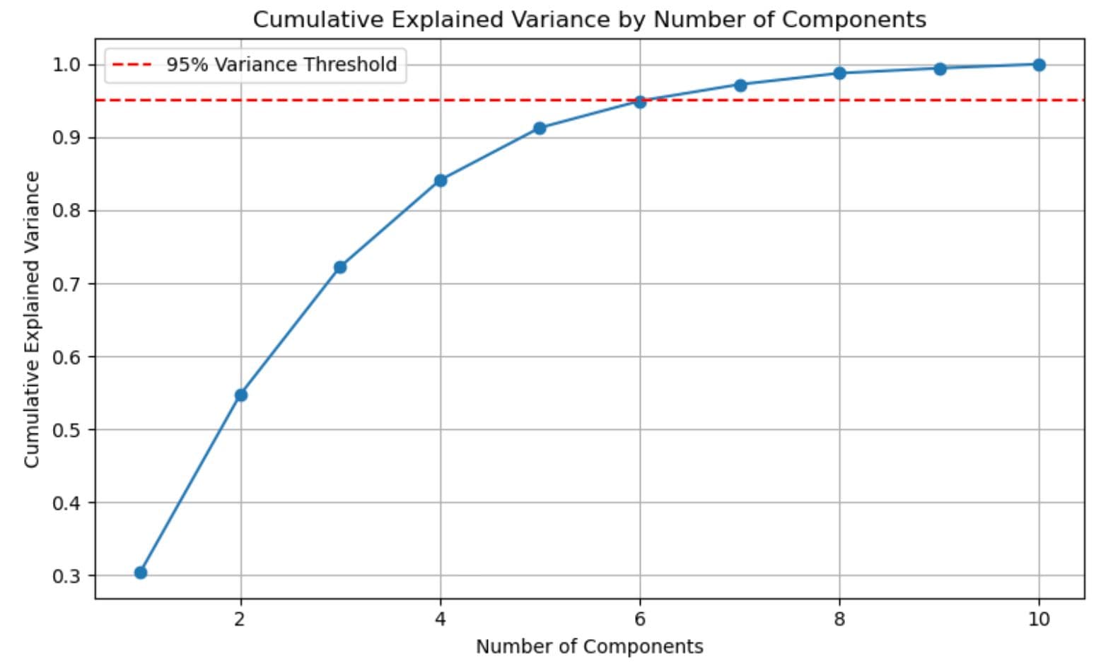
The line illustrates how much of the total variance is explained as more components are added.As shown above, just the first six components are sufficient to explain over 95% of the dataset.

This means instead of using all features, we can keep only those six components and still preserve almost all helpful information. That makes the data smaller, faster to process, and often better for modeling.

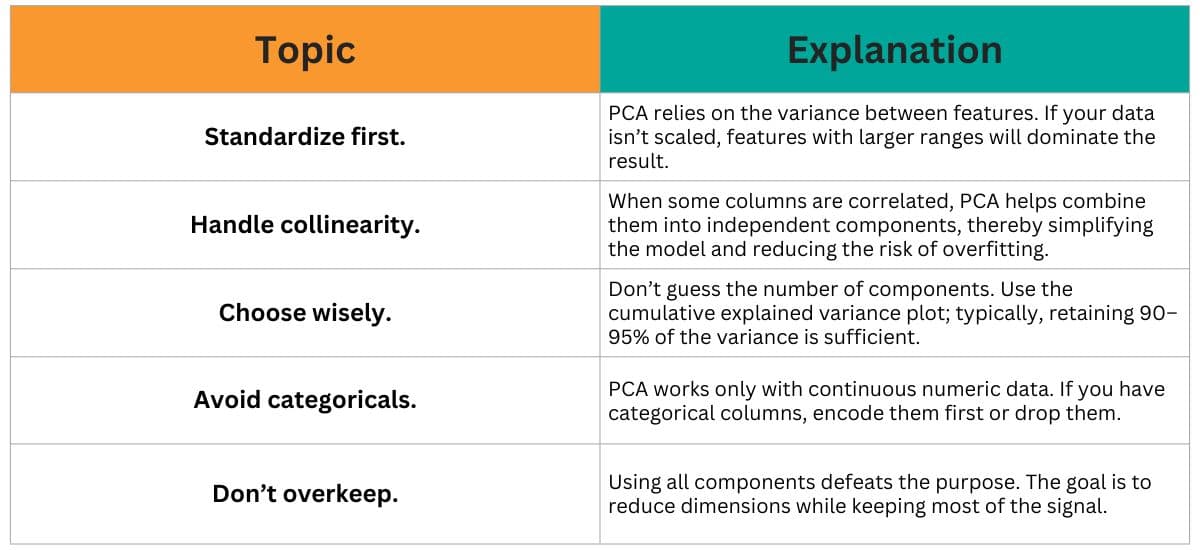
Common Pitfalls & Best Practices

PCA is robust, but it's easy to misuse. Here are a few key points to consider when using it in real-world projects.

Final Thoughts

One of the easiest and most valuable tools in your data science toolbox is PCA analysis in Python. It cuts down on noise, accelerates models, and highlights the most essential parts of your data.

While PCA isn’t always necessary, it can be especially useful when your dataset has many features or when those features overlap in the information they provide. With the right approach, PCA can make your models simpler, faster, and often more effective.