Implementing a Logit Model in R Effectively

How to build and interpret a logit model in R to predict customer churn: data preparation, modeling, and evaluation

Many models are overly complex for problems that only require straightforward yes-or-no answers. Logit models offer a clear and easy-to-understand technique to deal with binary outcomes, such as predicting churn. In this article, we will explore the application of a logit model in R using real churn data from a Sony Research project.

What Is a Logit Model in R and When to Use It?

A logit model is used to determine whether an event is true or false, such as whether a customer will churn or not.

Using the logistic function, it estimates how likely an observation is to belong to one of two groups. In R, the glm() function with family = binomial is used to perform this.

This is the standard syntax:

model <- glm(target_variable ~ predictor1 + predictor2, data = your_data, family = binomial)

The model illustrates how different factors influence the likelihood of an event, allowing you to convert its results into precise probabilities.

Visualizing the Logit Model in R

To understand what a logit model really does, it's helpful to visualize the logistic (sigmoid) function and how it maps any input into a probability between 0 and 1.

Below is the shape of the logistic function:

ggplot(df, aes(x = customer.service.calls, y = churn)) +
  geom_jitter(width = 0.3, height = 0.05, alpha = 0.3) +
  stat_smooth(method = "glm", method.args = list(family = "binomial"), se = TRUE) +
  labs(title = "Churn vs. Customer Service Calls (Logit Fit)",
       x = "Customer Service Calls",
       y = "Pr(Churn)") +
  scale_y_continuous(labels = scales::percent_format(accuracy = 1)) +
  theme_minimal(base_size = 12)

Here is the output.

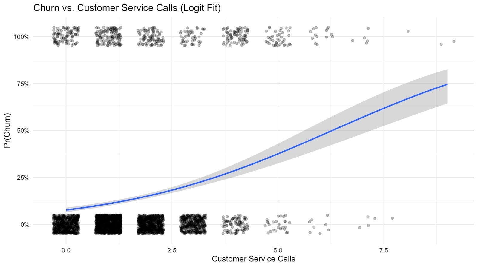
This S-shaped curve is great for predicting churn because it easily maps input values to probabilities between 0 and 1. This makes it perfect for situations where the outcome is either "churn" or "no churn".

Using a Real Data Project from Sony to Apply a Logit Model in R

In this data project, Sony asked you to:

• Perform explanatory analysis
• Prepare the data to build a predictive model
• Build a predictive model to predict customer churn
• Evaluate the model performance
• Discuss potential issues with deploying the model in production.

In this article, we will cover all the steps except the last one.

Data Exploration

In this step, we will explore the data. First, let’s load the dataset and display the first few rows by using the following code.

library(tidyverse)

df <- read.csv("Data_Science_Challenge.csv", stringsAsFactors = FALSE)

head(df, 5)

Here is the result.

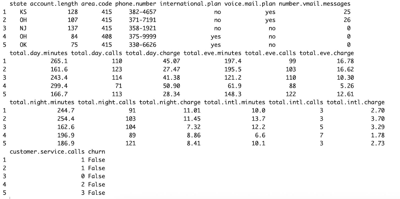
The dataset includes customer information (State, Area code, Phone number, Account length), plans (International plan, Voicemail plan), usage metrics for Day, Evening, Night, and International calls (minutes, calls, charges), other factors (Voicemail messages, Customer service calls), and the target variable (Churn).

Preparing Data for a Logit Model in R

You need to clean up the data first before you can build a model.

This involves converting categorical variables, removing identifiers, and, if necessary, scaling values.

This is what we'll do in R:

library(tidyverse)

df <- read.csv('/Users/learnai/Downloads/datasets 2/Data_Science_Challenge.csv')

df <- df %>%
  select(-c(state, phone.number))

df$international.plan <- ifelse(df$international.plan == "yes", 1, 0)
df$voice.mail.plan <- ifelse(df$voice.mail.plan == "yes", 1, 0)

df$churn <- as.integer(df$churn == "True")

df <- df %>%
  mutate(area_code = as.factor(area.code)) %>%
  select(-area.code) %>%
  mutate(across(area_code, as.factor)) %>%
  bind_cols(model.matrix(~ area_code - 1, data = .)) %>%
  select(-area_code)

str(df)

Here is the output.

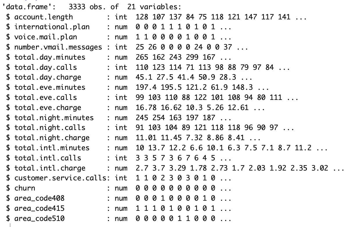
The dataset is now prepared to fit the logit model since all of the variables are now numeric.

Implementing a Logit Model in R Using glm()

Putting together a logit model is easy once the data is ready. To do a logistic regression, you just need to enter your formula, your dataset, and the value family = binomial.

For our churn forecast case, we will use all of the other columns to predict the churn variable.

The model can be made in this way:

logit_model <- glm(churn ~ international.plan + voice.mail.plan + customer.service.calls + total.day.charge,
                   data = df,
                   family = binomial)

summary(logit_model)

Here is the output.

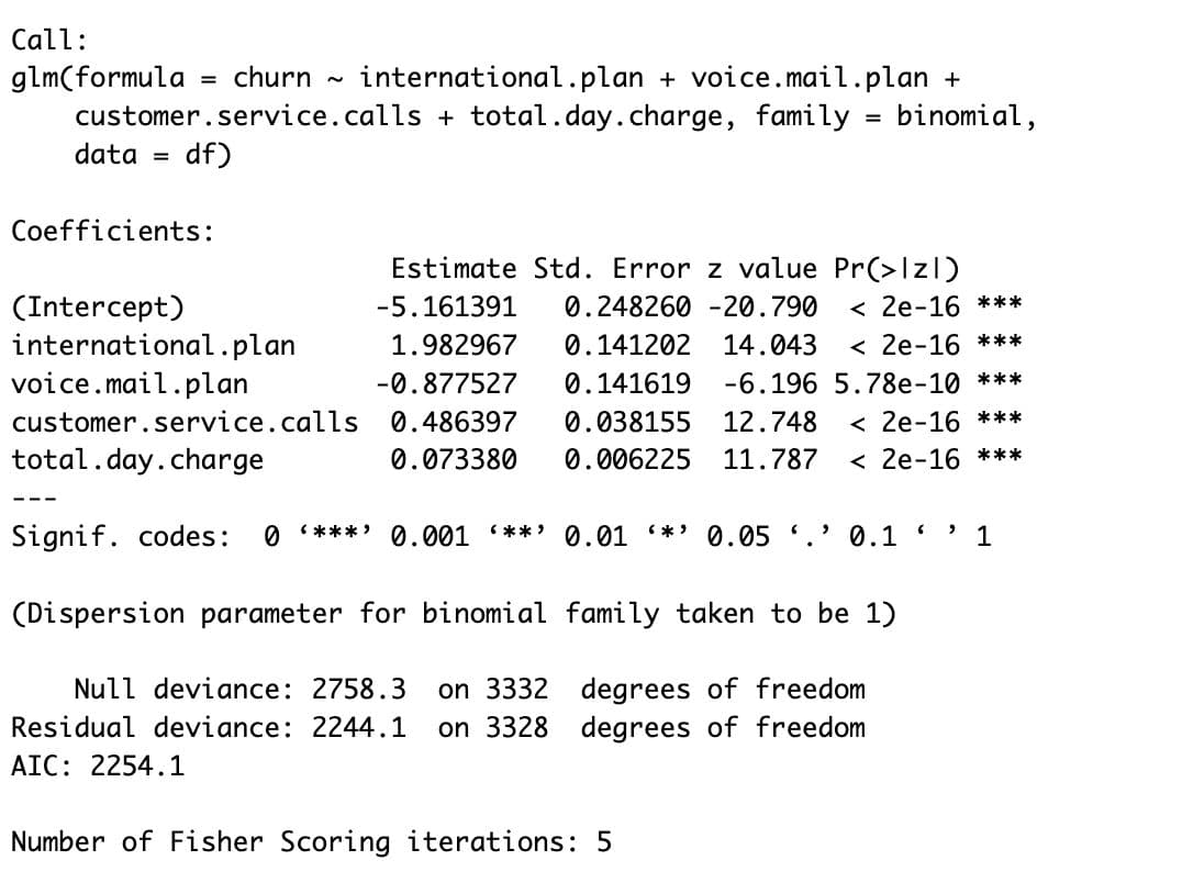
Now, let’s evaluate the result.

Visualizing the Predicted Probabilities

Let’s also look at the distribution of predicted churn probabilities, split by actual churn vs. no churn:

df$pred <- predict(logit_model, type = "response")

ggplot(df, aes(x = pred, fill = factor(churn))) +
  geom_histogram(position = "identity", alpha = 0.5, bins = 30) +
  labs(title = "Predicted Churn Probability by Actual Class",
       x = "Predicted Probability",
       fill = "Actual Churn") +
  theme_minimal(base_size = 12)

Here is the output.

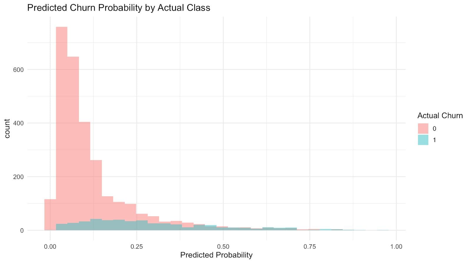
Most non-churners are confidently predicted with low probabilities, while churners are more spread out, showing why the model struggles to catch them. This explains the high accuracy but low recall we observed earlier.

Interpreting the Model Output

After reviewing the output in the previous section, let's figure out what the model's results mean and what they tell us about churn.

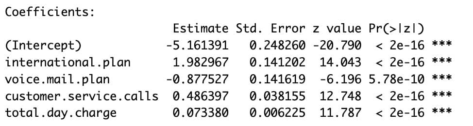
• international.plan: +1.98
  • Customers with international plans are much more likely to churn. This is one of the strongest indicators in the model.
• voice.mail.plan: −0.88
  • Voicemail plans make it much less likely that customers will leave. It could mean that these customers are more interested or get texts more often.
• customer.service.calls: +0.49
  • The chance of churn increases as the number of help calls increases. This is a standard sign that users are unhappy or that problems have not been fixed.
• total.day.charge: +0.07
  • There is a higher chance of churn when daily charges are higher.

The extremely low p-values for each of these variables testify to their statistical significance. These insights can directly inform churn mitigation strategies.

Evaluating Model Performance

We must evaluate the model's ability to forecast churn after fitting it. This can be accomplished in R by computing standard classification measures such as accuracy, precision, recall, and F1-score using a confusion matrix.

For illustration, let's begin by making predictions using the same dataset:

predictions <- predict(logit_model, type = "response")

predicted_class <- ifelse(predictions > 0.5, 1, 0)

table(Predicted = predicted_class, Actual = df$churn)

Here is the output.

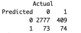
Here’s how to interpret it:

• True Negatives (2777): Predicted no churn, and the customer stayed.
• False Positives (73): Predicted churn, but the customer stayed.
• False Negatives (409): Predicted no churn, but the customer left.
• True Positives (74): Predicted churn, and the customer left.

Additional Performance Metrics

To better assess our model's predictive power, we may compute a few critical performance indicators in addition to the confusion matrix.

To calculate them in R, follow these steps:

library(caret)

conf_matrix <- confusionMatrix(
  factor(predicted_class),
  factor(df$churn),
  positive = "1"   
)

conf_matrix

Here is the output.

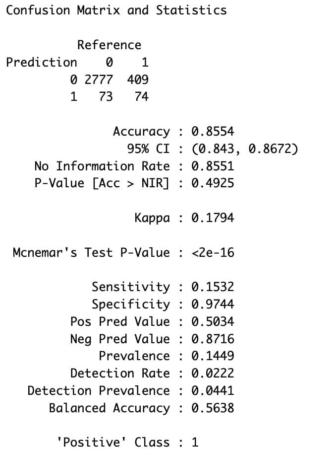
Here is how to interpret them:

• Accuracy (85.5%)
  • The model correctly predicts whether a customer will churn or not 85.5% of the time.
• Precision (50.3%) (a.k.a. Pos Pred Value)
  • When the model predicts churn, it is correct about half the time.
• Recall (15.3%) (a.k.a. Sensitivity)
  • The model successfully identifies only 15.3% of customers who churn, meaning it misses most churners.
• Specificity (97.4%)
  • The model correctly identifies 97.4% of customers who stay.
• Negative Predictive Value (87.2%)
  • When the model predicts no churn, it is correct 87.2% of the time.
• Balanced Accuracy (56.4%)
  • The average of sensitivity (recall for churn) and specificity (recall for stay) shows moderate performance overall, but it is not reliable enough for business decisions yet.

Conclusion

Using real data from Sony, this project showed how a simple logit model can be used to predict when a customer will leave. We prepared the dataset and then built and analyzed a logistic regression model that showed the main reasons why people leave their plans, such as having an international plan or calling customer service frequently.

The model was fairly accurate overall but it has room for improvement. Nevertheless, it provided clear and actionable insights, showing that even simple models can support strategic decision-making when properly built and interpreted.