Data Project from DoorDash – Delivery Duration Prediction

Here’s a data project that has been used as a take-home assignment by DoorDash to test your data science (Python, more precisely) skills.

Doordash is a company that allows customers to order food online and delivers it to their location. Delivery time is important for customers and businesses because it can affect customer satisfaction in the food and delivery industry. Ensuring timely delivery is crucial in the food delivery industry.

By predicting the time taken from when a consumer places an order to when it is delivered, DoorDash can better inform its customers and improve their satisfaction.

In this data project, we will handle the task of predicting the total delivery duration for orders placed on DoorDash.

The link to this project is here:
https://platform.stratascratch.com/data-projects/delivery-duration-prediction

When solving this take-home assignment, we will start with data preparation and modeling.

Then we will check the collinearity by using a heatmap and remove the redundancies.

The third stage is to look for multicollinearity and select the features according to the Ginis importance index.

As a final step, we will apply different models and techniques to find the model that fits best. Actually, we will apply the Deep Learning model here.

We will discuss the results of our analysis and conclude with some final thoughts on the task of delivery duration prediction for DoorDash.

Part 1: Data Preparation For Modeling

Now, let’s start with exploring data. Feel free to make it easier by watching our video focusing on this step:

Data Exploration

Import Libraries

Let’s first import the libraries. We will do data manipulation and work with arrays, that’s why we load pandas and NumPy. Also, we will draw a graph by using matplotlib and seaborn.

import pandas as pd
import numpy as np
import matplotlib.pyplot as plt
import seaborn as sns

Read and View Data

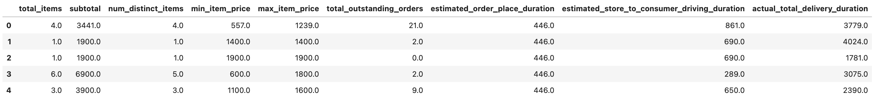
Here we will read our data from the CSV file and then we will look at the first rows of our data.

historical_data = pd.read_csv("historical_data.csv")
historical_data.head()

Here is our output.

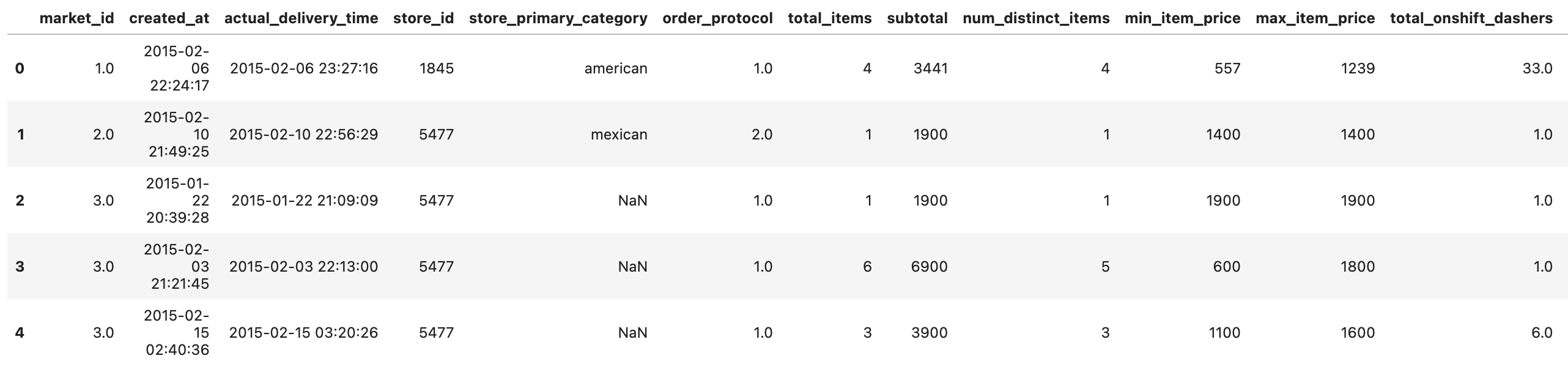
Data Exploration

After that, let’s use the info function to see the datatypes, lengths, and memory usage of our data frame.

historical_data.info()

Here is our data frame.

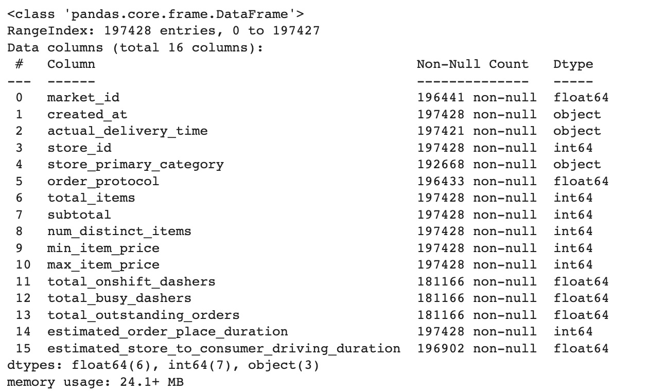
Here we can see the differences between the shapes of our features. That means we have a lot of missing & na values. Also, if we use categorical data in our model, we should turn them into dummy variables because machine learning models accept numerical data. Yet, variables like market_id are not effective for us, so that they can be removed.

Format Your Columns

We will do calculations by using the DateTime data type. To do that, we should convert our columns format. So we will use the datetime library. First, we will import the datetime library and use the to_datetime() function to change the created_at column and actual_delivery_time.

from datetime import datetime 
historical_data["created_at"] = pd.to_datetime(historical_data['created_at'])
historical_data["actual_delivery_time"] = pd.to_datetime(historical_data['actual_delivery_time'])

Create New Features

We do not have a variable that the problem wants us to create, so we should calculate it by using our features. Here, we will create three different features, one of them is our target variable, which is the actual total delivery duration. Let’s do it.

Actual Total Delivery Duration

We will subtract created_at from the actual_delivery_time to find the actual total delivery duration. After that, we will transform it into seconds by using the total_seconds() function. Let’s do it and look first rows of our data frame.

historical_data["actual_total_delivery_duration"] = (historical_data["actual_delivery_time"] - historical_data["created_at"]).dt.total_seconds()
historical_data.head()

Here is the output of our code.

Estimated Non-Prep Duration

Alright, we can think of the delivery process by splitting it into two subsections preparation and non-preparation time. We will add estimated_store_to_customer_driving_duration to estimated_order_place_duration. Let’s do it with the following code and look first rows of our data frame.

historical_data['estimated_non_prep_duration'] = historical_data["estimated_store_to_consumer_driving_duration"] + historical_data["estimated_order_place_duration"]
historical_data.head()

Here is the output of our code.

Busy_dashers_ratio

To make the comparison more meaningful, we will create a new variable called 'busy_dashers_ratio'. This variable will represent the proportion of busy dashers when an order was placed, expressed as a percentage of the total number of dashers working the shift at that time.

historical_data["busy_dashers_ratio"] = historical_data["total_busy_dashers"] / historical_data["total_onshift_dashers"]

Data Preparation

In this step, we will prepare our data for building a machine-learning model in the next stages. To do that, let’s look at three categorical columns to decide whether we will turn these into numbers.

# check ids and decide whether to encode or not
historical_data["market_id"].nunique()
historical_data["store_id"].nunique()
historical_data["order_protocol"].nunique()

Our code outputs 6, 6743, and 7, respectively. Store id columns have too many (6743) different options, so we remove that option. Yet, market_id and order_id can turn into numerical variables.

Here we will first find a unique store id and assign them to store_id_unique and then find the most frequent category in the second step.

store_id_unique = historical_data["store_id"].unique().tolist()
store_id_and_category = {store_id: historical_data[historical_data.store_id == store_id].store_primary_category.mode() 
                         for store_id in store_id_unique}

Then we will use a custom function to fill these values into our data frame by using it with the apply method afterward.

def fill(store_id):
    """Return primary store category from the dictionary"""
    try:
        return store_id_and_category[store_id].values[0]
    except:
        return np.nan

# fill null values
historical_data["nan_free_store_primary_category"] = historical_data.store_id.apply(fill)

Alright, now our categorical variable is ready to be turned into numerical by using the get_dummies pandas function.

Dummy Variables

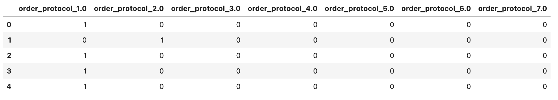
Here, we will create dummy variables for order_protocol and market_id and view the first rows of the data frame.

order_protocol_dummies = pd.get_dummies(historical_data.order_protocol)
order_protocol_dummies = order_protocol_dummies.add_prefix('order_protocol_')
order_protocol_dummies.head()

Here is the output.

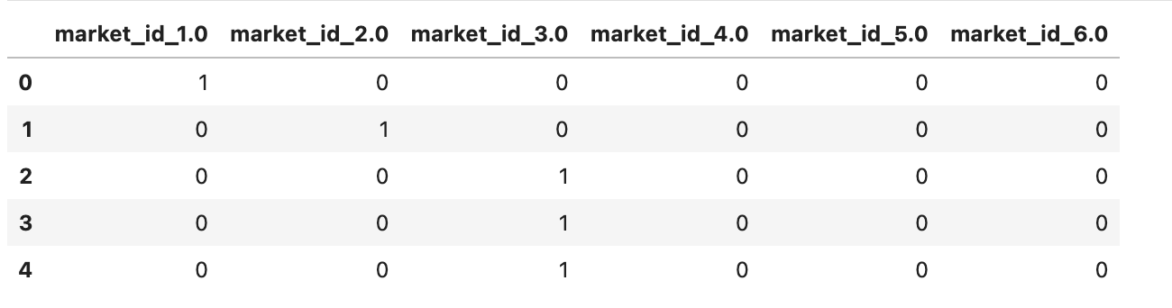
# create dummies for market_id
market_id_dummies = pd.get_dummies(historical_data.market_id)
market_id_dummies = market_id_dummies.add_prefix('market_id_')
market_id_dummies.head()

Here is the output.

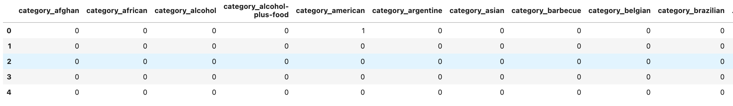
Alright, now we will create dummies for store_primary_category.

store_primary_category_dummies = pd.get_dummies(historical_data.nan_free_store_primary_category)
store_primary_category_dummies = store_primary_category_dummies.add_prefix('category_')
store_primary_category_dummies.head()

Here is our output.

Data Frame Restructuring

At this stage, let’s restructure our data frame by removing the original columns and replacing them with the dummies variable by using the concat() function.

train_df = historical_data.drop(columns = ["created_at", "market_id", "store_id", "store_primary_category", "actual_delivery_time", "nan_free_store_primary_category", "order_protocol"])
train_df.head()

Here is our output.

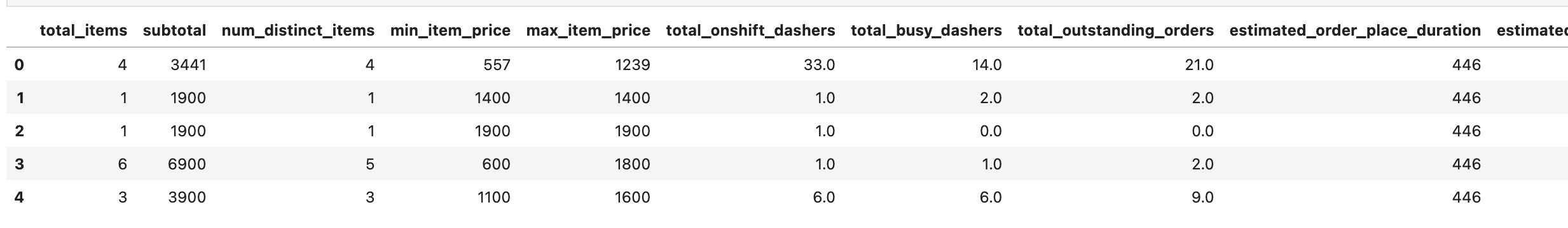
train_df = pd.concat([train_df, order_protocol_dummies, market_id_dummies, store_primary_category_dummies], axis=1)
train_df = train_df.astype("float32")
train_df.head()

Here is our output.

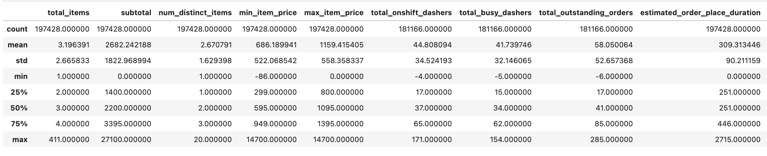
Since we have 100 columns, it might be hard to grasp them just by looking into the first rows of our DataFrame, so you can dig deeper by using different statistical functions.

train_df.describe()

Here is the output.

train_df["busy_dashers_ratio"].describe()

Here is the output.

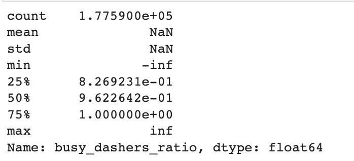
Check infinity values

Here, we can see the inf values. They happen because we calculated the busy dasher's ratio by doing the dividing operation. And if you divide some number by zero, the output will be inf if your number is positive. If your number is negative, then it will be -inf.

So to get rid of such values, we will use three different functions that aim to find inf values in our DataFrame.

np.where(np.any(~np.isfinite(train_df),axis=0) == True)

Now we can replace these inf values with the NaN values and drop them. Let’s look at the shape of our DataFrame to see how many rows are left.

train_df.replace([np.inf, -np.inf], np.nan, inplace=True)
train_df.dropna(inplace=True)
train_df.shape

Here is the output.

As you can see, in the beginning, some of our columns had up to 197428 rows. It looks like we removed 20.358 rows along the way of the data preparation for modeling.

Now, let’s double-check whether or not our DataFrame still contains missing values.

train_df.isna().sum().sum()

Alright, it looks like we removed all NAs successfully.

Part 2: Collinearity and Removing Redundancies

Here, we will focus on collinearity and removing it, like drawing a heatmap and writing a custom function after.

Here’s our video to help you better understand this section.

Collinearity occurs when two or more predictor variables in a regression model are highly correlated with each other. This can lead to problems in interpreting the results of the model, as the coefficients of the correlated variables may be unstable and difficult to interpret.

In addition, collinearity can affect the model’s predictive power, as it can reduce the variance of the coefficients and increase the standard errors. This leads to a decrease in the overall model accuracy.

To address collinearity, one approach is to reduce the dimensionality of the data by selecting a subset of variables that are not highly correlated with each other. One way to do this is by using a correlation matrix, which shows the correlation between all pairs of variables in the DataFrame. Also, a heatmap can be used to visualize the correlations and a mask can be used to identify variables that are highly correlated and may need to be removed from the model.

Other approaches to addressing collinearity are using regularization techniques such as Ridge or Lasso regression or using principal component analysis, which we will go through in Part 3.

In this data project we will use the diagonal heatmap.

Diagonal Heatmap

We will apply the mask to our heatmap to slice it diagonally after we draw it. To create a mask, we will create an array filled with ones.  We will then assign the upper side of the array a value of 1 and the lower side a value of 0, and apply the mask by setting all values to 1. Once the mask has been created, we will use the seaborn’s diverging_palette to show the density using different color tones. Next, we will use the seaborn heatmap() method, along with the arguments ‘corr’ and ‘mask’ to complete the process.

Here is the code.

corr = train_df.corr()
mask = np.triu(np.ones_like(corr, dtype=bool))

f, ax = plt.subplots(figsize=(11, 9))

cmap = sns.diverging_palette(230, 20, as_cmap=True)

sns.heatmap(corr, mask=mask, cmap=cmap, vmax=.3, center=0,
            square=True, linewidths=.5, cbar_kws={"shrink": .5})

The code will return this heatmap.

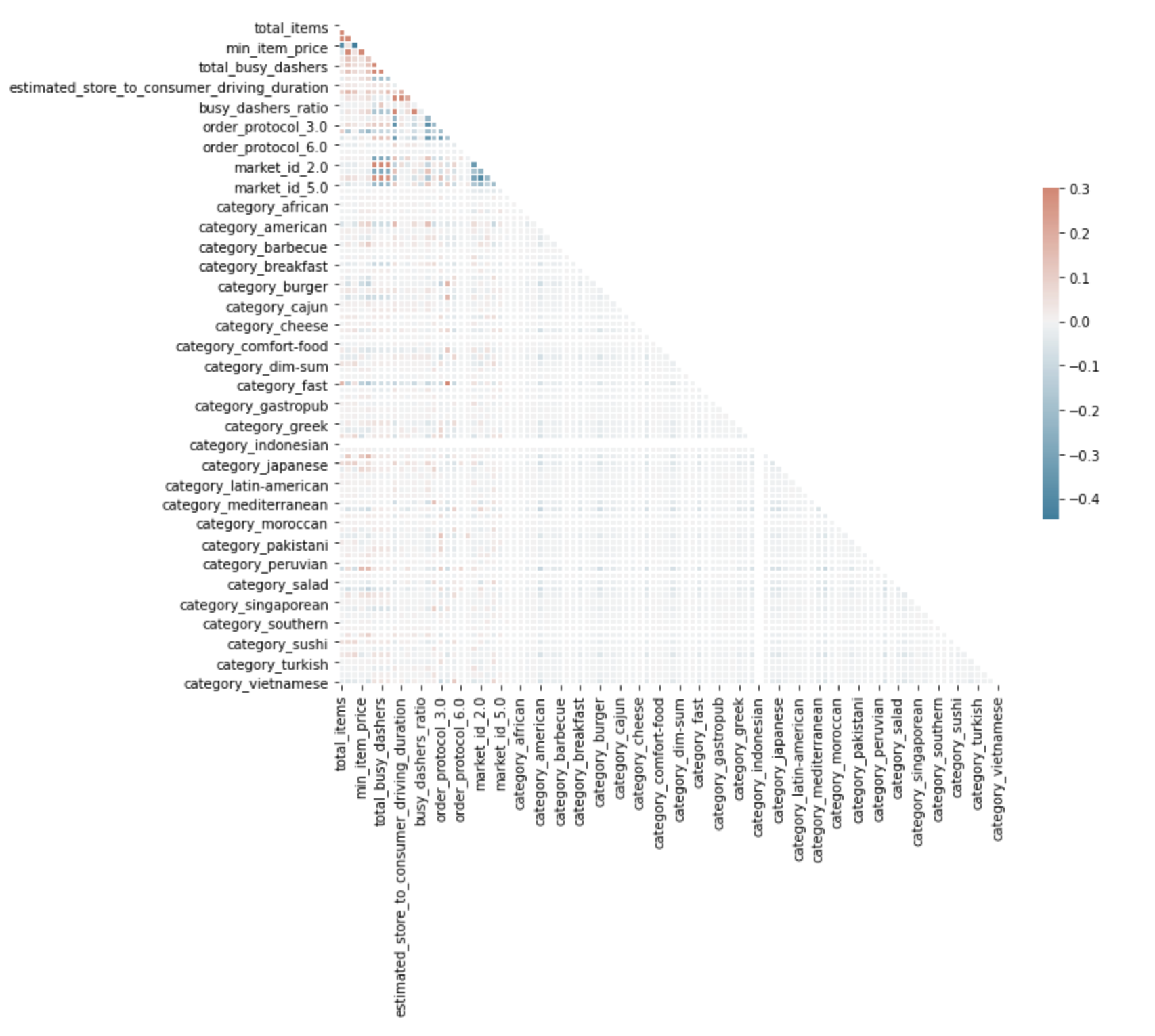
It looks like we have a problem with one of our features, category_indonesioan.

So let’s look closely at it.

train_df['category_indonesian'].describe()

Here is the output.

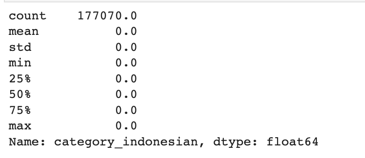
It has 177,070 zeros, so we can drop this one.

Also, what would have happened if we had not applied the mask? In the below image, you can see two heatmaps. The right one is without the applied mask.

Let’s go to the part where we will find redundant pairs by defining a custom function first.

Finding Redundant Pairs

Here, we will define two functions. The first one helps you create a function that will eventually pair the columns from the DataFrame.

def get_redundant_pairs(df):
    pairs_to_drop = set()
    cols = df.columns
    for i in range(0, df.shape[1]):
        for j in range(0, i+1):
            pairs_to_drop.add((cols[i], cols[j]))
    return pairs_to_drop

Removing Redundant Pairs

The second function is for calculating the correlation. It uses the first function that makes pairs and eventually removes them.

def get_top_abs_correlations(df, n=5):
    au_corr = df.corr().abs().unstack()
    labels_to_drop = get_redundant_pairs(df)
    au_corr = au_corr.drop(labels=labels_to_drop).sort_values(ascending=False)
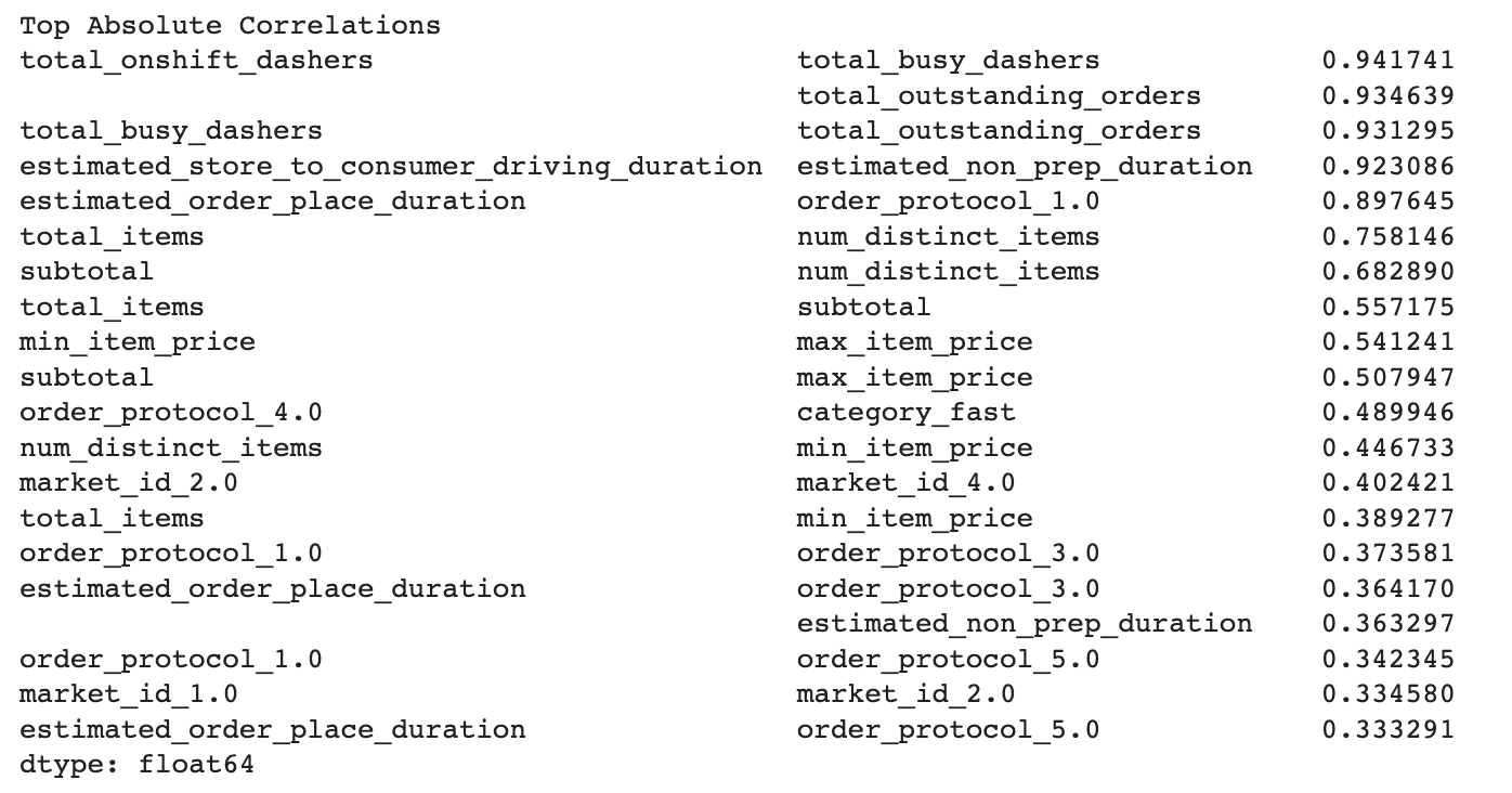
    return au_corr[0:n]

Running Code

Alright, let’s run the above code and see its output.

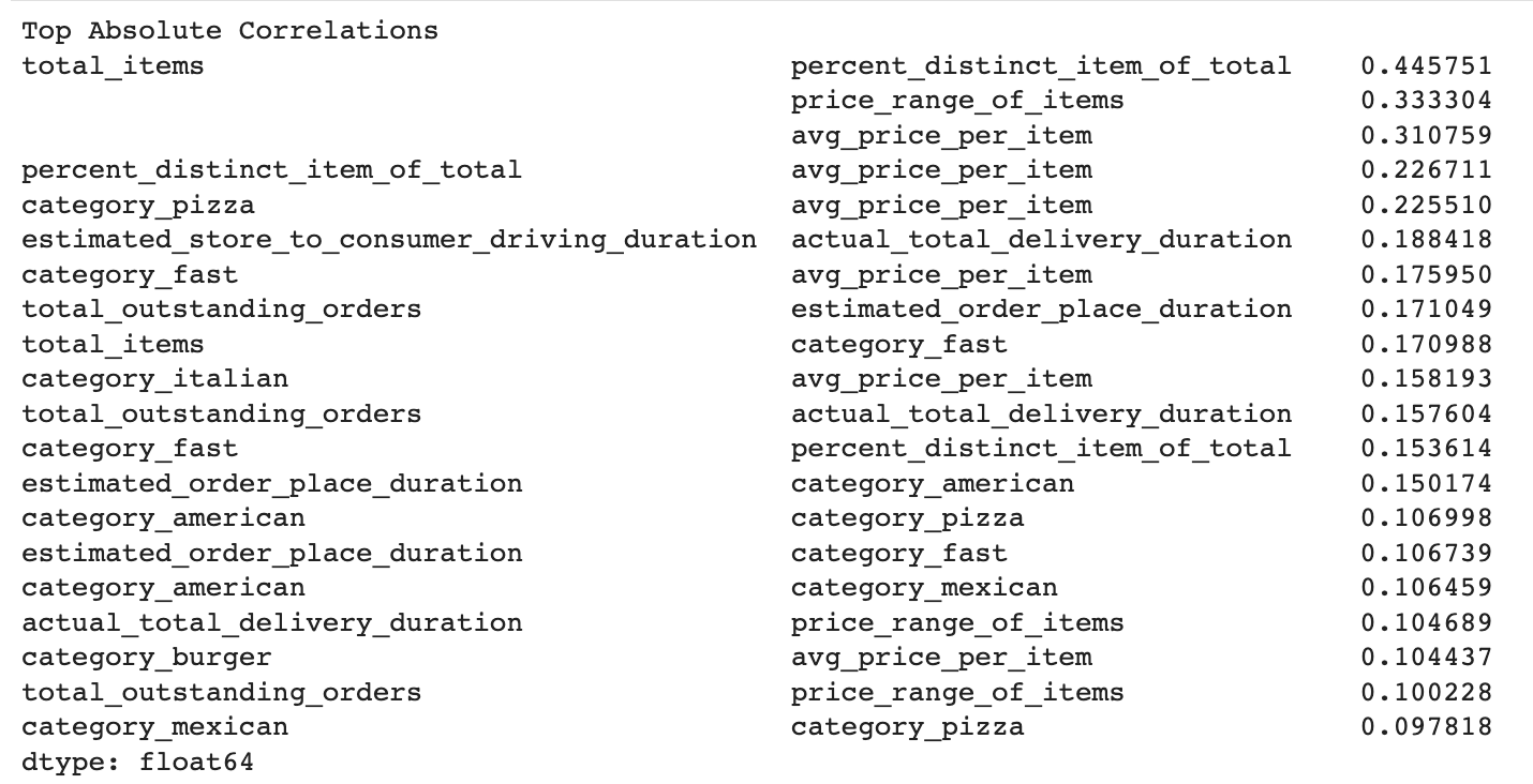
print("Top Absolute Correlations")
print(get_top_abs_correlations(train_df, 20))

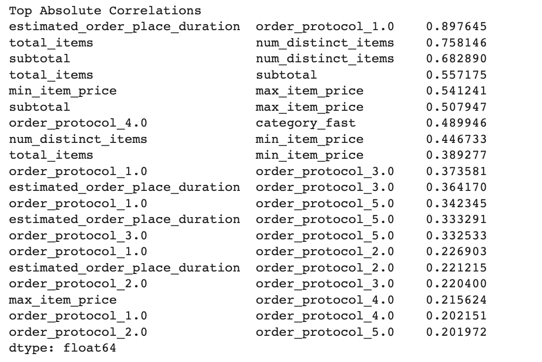
Here is our output. It contains pairs that have high correlations, which might cause collinearity.

Concatenate With The Dummies

We worked with the numerical features to find the correlation. Now, we will merge our numerical features with the dummy variables, but here we will use the iterative method to find the best model to avoid correlation.

First, let’s don’t concat order_protocol_dummies from all dummy DataFrames. After that, we will look at the rows of our data frame.

train_df = historical_data.drop(columns = ["created_at", "market_id", "store_id", "store_primary_category", "actual_delivery_time", 
                                        "nan_free_store_primary_category", "order_protocol"])
train_df = pd.concat([train_df, store_primary_category_dummies], axis=1)
train_df = train_df.drop(columns=["total_onshift_dashers", "total_busy_dashers",
   "category_indonesian", "estimated_non_prep_duration"])
train_df = train_df.astype("float32")

train_df.replace([np.inf, -np.inf], np.nan, inplace=True)
train_df.dropna(inplace=True)
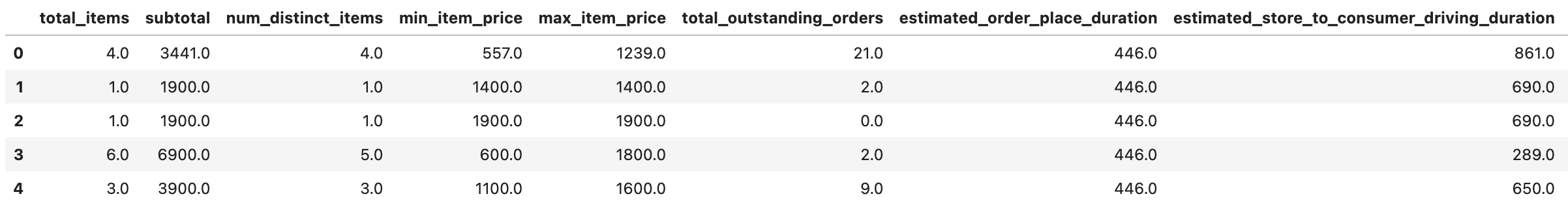
train_df.head()

Here is the output of our code.

Correlated features

Now, let’s rerun our custom function.

print("Top Absolute Correlations")
print(get_top_abs_correlations(train_df, 20))

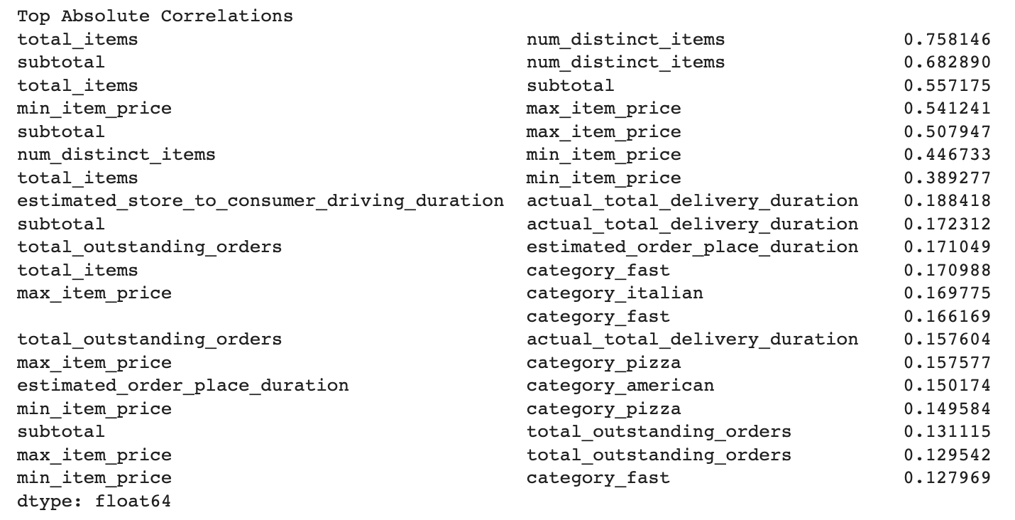
Here is our output.

Concatenate again

Now, let’s concatenate the dummies without adding order_protocl_dummies.

train_df["percent_distinct_item_of_total"] = train_df["num_distinct_items"] / # drop created_at, market_id, store_id, store_primary_category, actual_delivery_time, order_protocol
train_df = historical_data.drop(columns = ["created_at", "market_id", "store_id", "store_primary_category", "actual_delivery_time", 
                                        "nan_free_store_primary_category", "order_protocol"])
train_df = pd.concat([train_df, store_primary_category_dummies], axis=1)
train_df = train_df.drop(columns=["total_onshift_dashers", "total_busy_dashers",
                                  "category_indonesian", 
                                  "estimated_non_prep_duration"])
train_df = train_df.astype("float32")
train_df.replace([np.inf, -np.inf], np.nan, inplace=True)
train_df.dropna(inplace=True)
train_df.head()

Here is our output.

Now, let’s see the correlation again.

train_df["percent_distinct_item_of_total"] = train_df["num_distinct_items"] / train_df["total_items"]
train_df["avg_price_per_item"] = train_df["subtotal"] / train_df["total_items"]
train_df.drop(columns =["num_distinct_items", "subtotal"], inplace=True)
print("Top Absolute Correlations")
print(get_top_abs_correlations(train_df, 20))

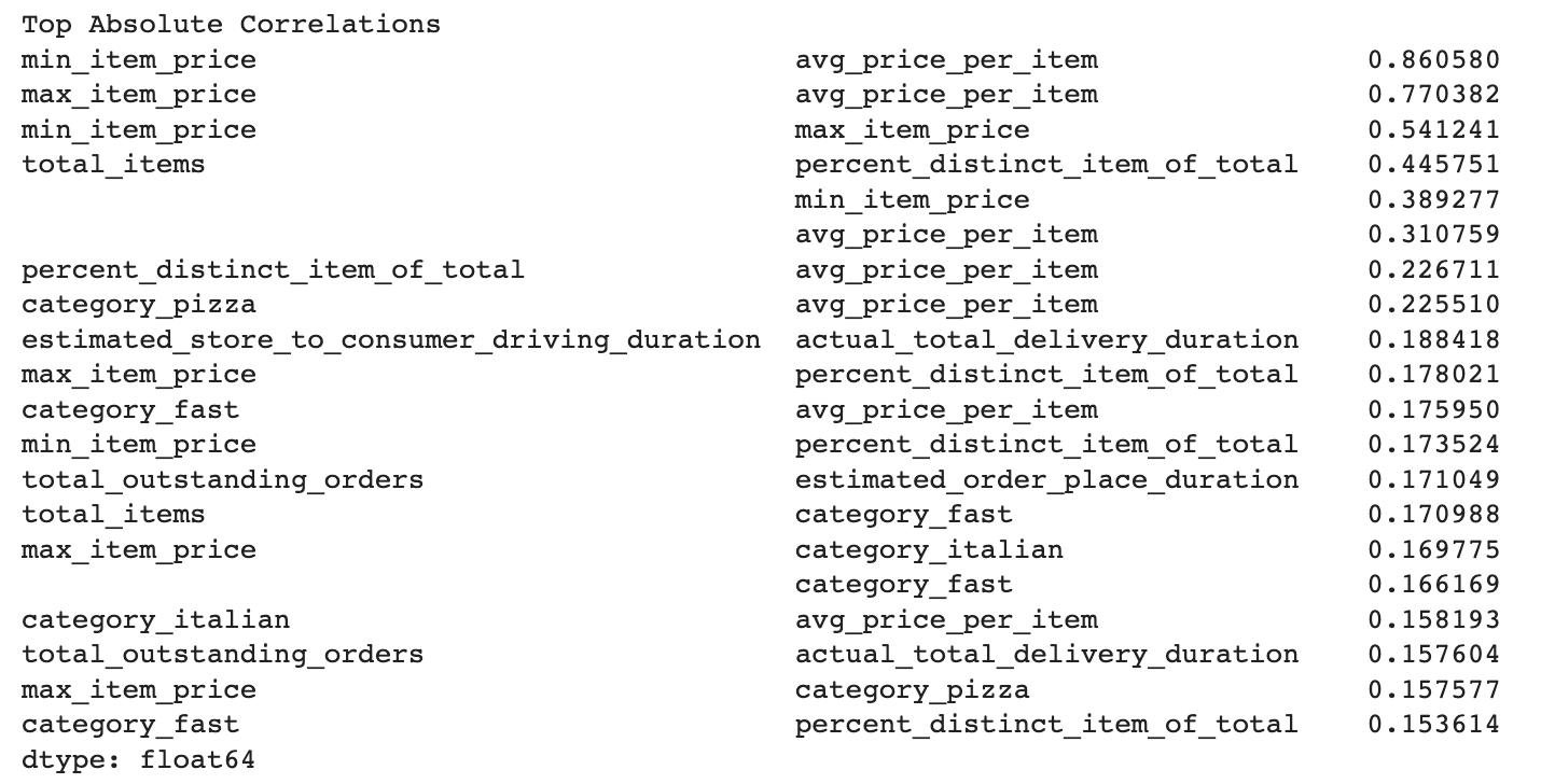
Here is our output.

Create New Features To Overcome The Multicollinearity Issues

Alright, it looks like we still have a problem. Let’s try to create a new variable, which might help us overcome this problem.

train_df["percent_distinct_item_of_total"] = train_df["num_distinct_items"] / train_df["total_items"]
train_df["avg_price_per_item"] = train_df["subtotal"] / train_df["total_items"]
train_df.drop(columns =["num_distinct_items", "subtotal"], inplace=True)
print("Top Absolute Correlations")
print(get_top_abs_correlations(train_df, 20))

Here is our output.

Again, do feature engineering by creating a new feature to overcome the issue of collinearity.

train_df["price_range_of_items"] = train_df["max_item_price"] - train_df["min_item_price"]
train_df.drop(columns=["max_item_price", "min_item_price"], inplace=True)
print("Top Absolute Correlations")
print(get_top_abs_correlations(train_df, 20))

Let’s see our output.

Okay, now we have solved the problem with correlation. Now, let’s look at the shape of our data frame again.

train_df.shape

Here is our output.

We used to have 100 columns, here we removed 18 columns.

Part 3: Multicollinearity and Feature Selection

Multicollinearity

In order to improve the interpretability and avoid overfitting in our regression analysis, it is important to solve the multicollinearity issue between our columns, which we will use for making predictions.

Multicollinearity happens when your variables are correlated with each other, making it more difficult to evaluate the results of the model and may lead to other issues.

You can follow this step in our video, too.

Multicollinearity Check with VIF

To find out the multicollinearity, we will develop the Variance Inflation Factor(VIF) method.  VIF measures how much the collinearity of a variable affects your regression model. We will remove any features with a VIF score above 20, as it shows a high level of multicollinearity.

To apply that process, we will create a custom function that calculates the VIF scores for each feature in our data frame. Then we will sort the values and create two columns that contain the feature names and corresponding VIF scores.

from statsmodels.stats.outliers_influence import variance_inflation_factor

def compute_vif(features):
    vif_data = pd.DataFrame()
    vif_data["feature"] = features
    vif_data["VIF"] = [variance_inflation_factor(train_df[features].values, i) for i in range(len(features))]
    return vif_data.sort_values(by=['VIF']).reset_index(drop=True)

Compute VIF Over the DataFrame

Now, let’s apply the VIF computation to all columns.

features = train_df.drop(columns=["actual_total_delivery_duration"]).columns.to_list()
vif_data = compute_vif(features)
vif_data

Dropping The Features

In this step, we will drop the highest VIF score by writing the while loop. It will first define the highest VIF features and then remove them.

multicollinearity = True

while multicollinearity:
    highest_vif_feature = vif_data['feature'].values.tolist()[-1]
    print("I will remove", highest_vif_feature)
    features.remove(highest_vif_feature)
    vif_data = compute_vif(features)
    multicollinearity = False if len(vif_data[vif_data.VIF > 20]) == 0 else True

selected_features = vif_data['feature'].values.tolist()
vif_data

Feature Selection

Feature selection is the process of identifying and removing redundant features from our data frame in order to improve the performance of a machine learning model.

There are many reasons why this is important. Primarily, it reduces the dimensionality of the DataFrame, which will help our algorithms work faster.

We will focus on two different methods to do that. The first one is Gini’s importance.

But before explaining this, let’s restart the procedure where we select our features and split them into test and training data.

from sklearn.ensemble import RandomForestRegressor
from sklearn.model_selection import train_test_split
X = train_df[selected_features]
y = train_df["actual_total_delivery_duration"]
X_train, X_test, y_train, y_test = train_test_split(
    X, y, test_size=0.2, random_state=42)

Gini-Importance

Here comes the tricky part. Let’s first learn what the Gini importance is. A Random Forest Regression allows us to measure the importance of our features by using the Gini importance, which calculates the importance of the features across all splits made by random forest regressor. Interesting, right?

Here, we will calculate the importance of each feature in our DataFrame and store the feature names and their importance values in a dictionary. That’s how we will select from the fraction of our DataFrame while applying the machine learning model in the next steps. Here is the code to do that.

feature_names = [f"feature {i}" for i in range((X.shape[1]))]
forest = RandomForestRegressor(random_state=42)
forest.fit(X_train, y_train)
feats = {} # a dict to hold feature_name: feature_importance
for feature, importance in zip(X.columns, forest.feature_importances_):
    feats[feature] = importance #add the name/value pair 

importances = pd.DataFrame.from_dict(feats, orient='index').rename(columns={0: 'Gini-importance'})
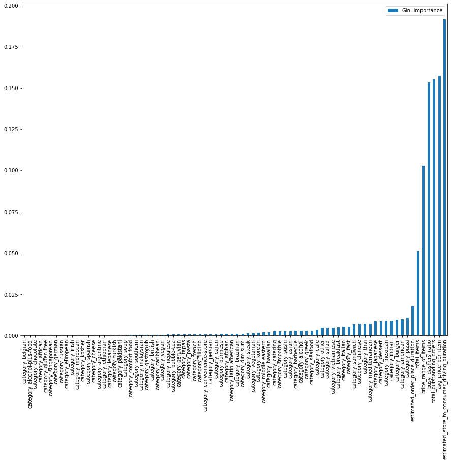
importances.sort_values(by='Gini-importance').plot(kind='bar', rot=90, figsize=(15,12))
plt.show()

Alright, here is the graph.

Sort by Gini Importance

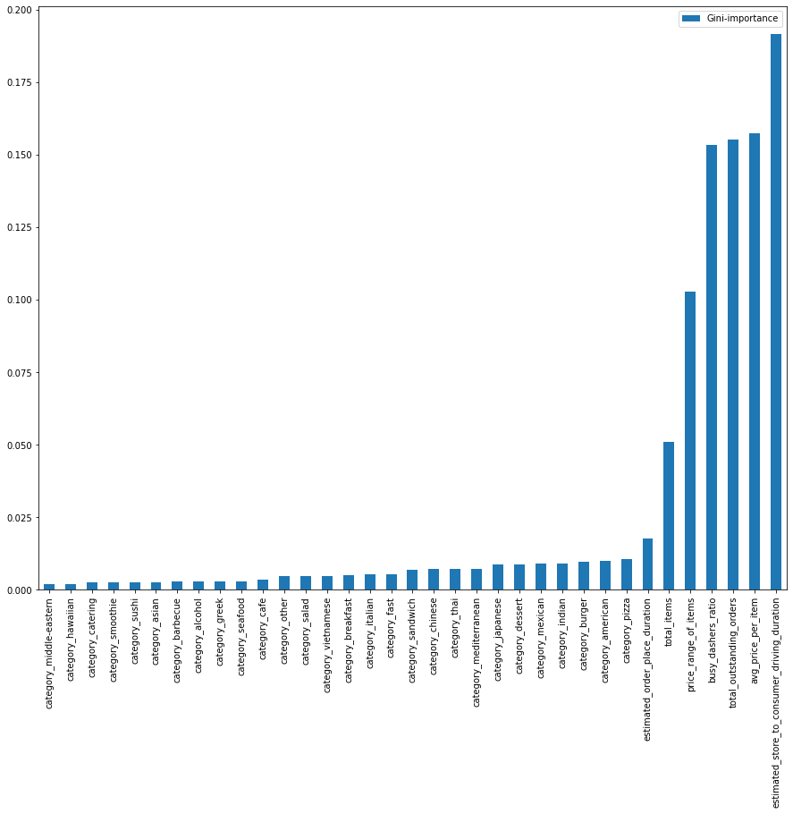
It looks a little bit complicated, so let’s minimize this graph by 35 of the best.

Let’s see the code.

importances.sort_values(by='Gini-importance')[-35:].plot(kind='bar', rot=90, figsize=(15,12))
plt.show()

Here is the output.

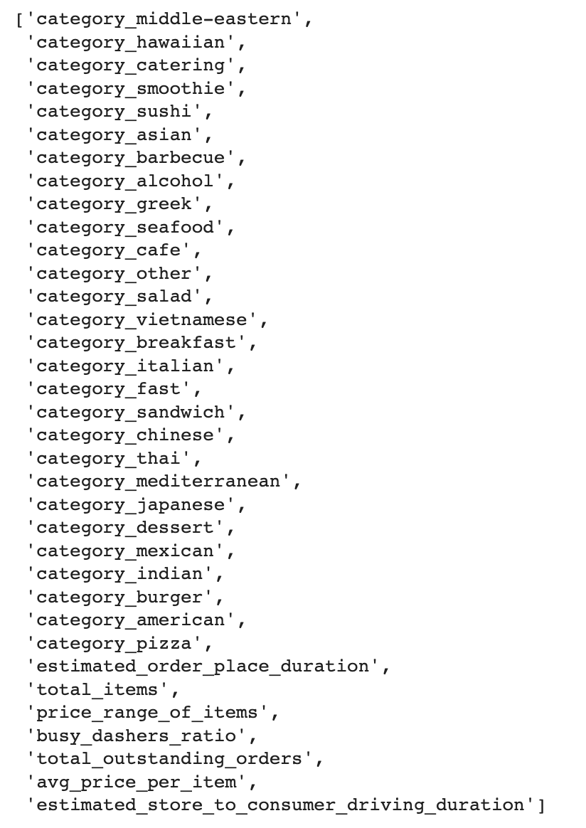
Selects by Gini Importance

Here, you can see that we can also find the list as a text.

Here is the code.

importances.sort_values(by='Gini-importance')[-35:].index.tolist()

Here is the output.

PCA

Principle component analysis is a technique for reducing the dimensionality of a DataFrame by identifying and removing redundant features. It is a common technique to reduce dimensionality and eliminate multicollinearity.

By using PCA, we can deduce how many features are needed to explain a certain percentage of the data in our DataFrame. This will help us find the optimum number of features to explain our data frame.

In our case, the goal is to find a way to enhance our model’s performance and improve our algorithm's speed by reducing the number of features from 80 to a more optimal level.

Here is the code to do that. We first import the necessary libraries. And then, we change our feature format, fit, and transform our features and fit it.

Next, we will draw a graph. Here is the code that does that.

from sklearn.decomposition import PCA
from sklearn.preprocessing import StandardScaler

X_Train = X_train.values
X_Train = np.asarray(X_Train)
X_std = StandardScaler().fit_transform(X_Train)
pca = PCA().fit(X_std)
plt.plot(np.cumsum(pca.explained_variance_ratio_))
plt.xlim(0,81,1)
plt.xlabel('Number of components')
plt.ylabel('Cumulative explained variance')
plt.show()

Here is the output.

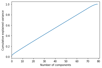
We can see that 60 features would explain 80% of our data frame. We already have 80 features, so it is okay. Yet if 10-20 features explain this percentage, we would remove our redundant features.

Scaler

In this step, we will define a custom function that will allow us to apply different scalers in our machine-learning process. Scaling is the process of transforming variables to the same scale, which will help our algorithm works faster.

There are two common methods for doing this, Min-Max Scaler and Standard Scaler.

Min-Max Scaler

The Min-Max Scaler scales the data between 0 and 1 by subtracting the minimum value and dividing it by the difference between the maximum and minimum values.

Standard Scaler

The Standard Scaler scales the data by subtracting the mean and dividing by the standard deviation.

Here is the custom function, which will apply the scaler by its name and transform it.

from sklearn.preprocessing import MinMaxScaler, StandardScaler

def scale(scaler, X, y):
    X_scaler = scaler
    X_scaler.fit(X=X, y=y)
    X_scaled = X_scaler.transform(X)
    y_scaler = scaler
    y_scaler.fit(y.values.reshape(-1, 1))
    y_scaled = y_scaler.transform(y.values.reshape(-1, 1))
    
    return X_scaled, y_scaled, X_scaler, y_scaler

We will apply this in the next section, let’s see the implementation.

Applying Scaler

X_scaled, y_scaled, X_scaler, y_scaler = scale(MinMaxScaler(), X, y)

X_train_scaled, X_test_scaled, y_train_scaled, y_test_scaled = train_test_split(
        X_scaled, y_scaled, test_size=0.2, random_state=42)

After scaling your data, you should inverse it to make your data the same. A custom function uses inverse_transform() function to do that.

Inverse Transform

from sklearn.metrics import mean_squared_error

def rmse_with_inv_transform(scaler, y_test, y_pred_scaled, model_name):
    y_predict = scaler.inverse_transform(y_pred_scaled.reshape(-1, 1))
    # return RMSE with squared False     
    rmse_error = mean_squared_error(y_test, y_predict[:,0], squared=False)
    print("Error = "'{}'.format(rmse_error)+" in " + model_name)
    
    return rmse_error, y_predict

Part 4: Classical Machine Learning

At this stage, we will follow the iterative process to find the best performance model, which means finding a model that has a lower RMSE error. We will use different models, scalers, and feature sets to do that. Then we will save these results in the list and turn this into a data frame for further analysis.

The Part 4 video is here to help you with this stage.

Machine Learning Models

Here is a custom function that will fit the models first, then calculate and print the evaluation metrics, train and test error, along with the trained model name with y_predict to then calculate these metrics for all models at once.

def make_regression(X_train, y_train, X_test, y_test, model, model_name, verbose=True):
    model.fit(X_train,y_train)
    y_predict=model.predict(X_train)
    train_error = mean_squared_error(y_train, y_predict, squared=False)
    y_predict = model.predict(X_test)
    test_error = mean_squared_error(y_test, y_predict, squared=False)
    if verbose:
        print("Train error = "'{}'.format(train_error)+" in " + model_name)
        print("Test error = "'{}'.format(test_error)+" in " + model_name)
    trained_model = model
    
    return trained_model, y_predict, train_error, test_error

Let’s load the libraries first.

from xgboost import XGBRegressor
from lightgbm import LGBMRegressor
from sklearn.neural_network import MLPRegressor
from sklearn import tree
from sklearn import svm
from sklearn import neighbors
from sklearn import linear_model

Alright, let’s continue creating dictionaries that will contain the different parameters. The parameters that we’ll test are shown below.

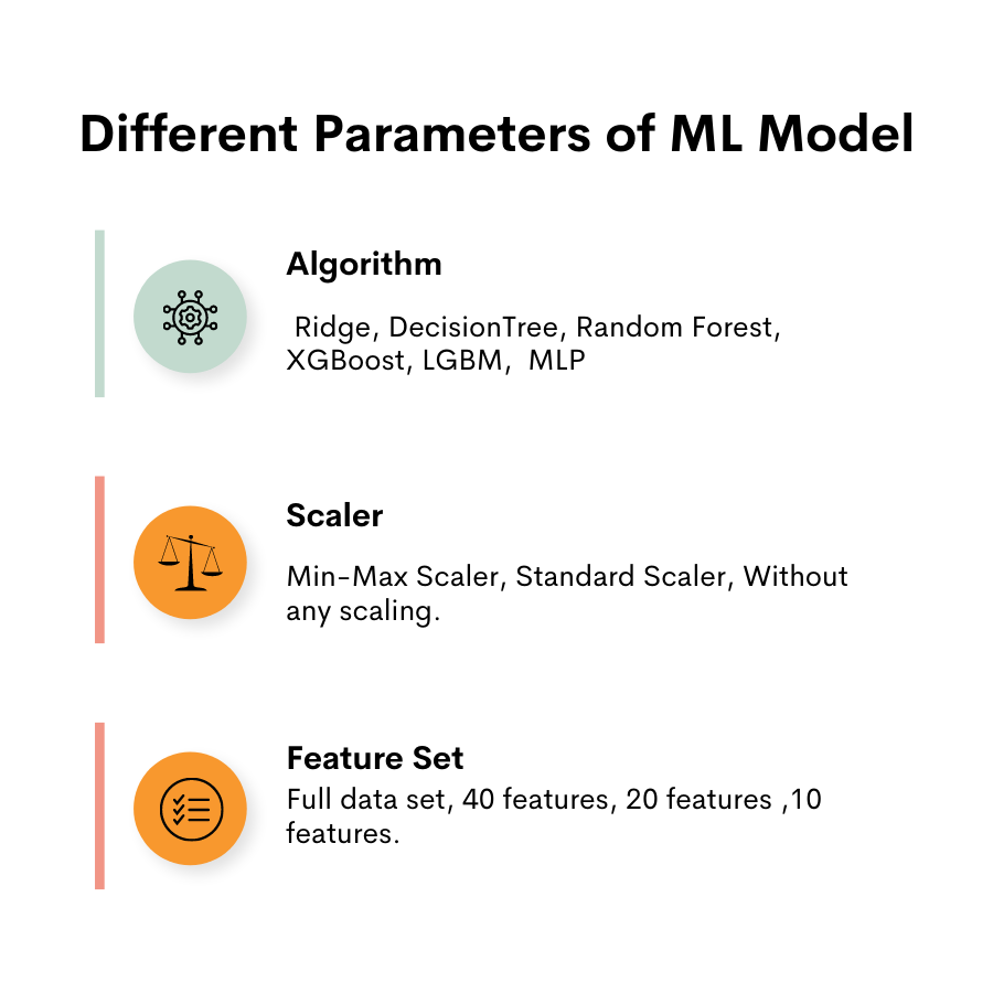
We will create pred_dict, which will store regression models, feature sets, scaler names, and RMSE for each model.

pred_dict = {
    "regression_model": [],
    "feature_set": [],
    "scaler_name": [],
    "RMSE": [],
}

Then we will define 6 different regression models starting with Ridge and ending with MLP.

regression_models = {
    "Ridge" : linear_model.Ridge(),
    "DecisionTree" : tree.DecisionTreeRegressor(max_depth=6),
    "RandomForest" : RandomForestRegressor(),
    "XGBoost": XGBRegressor(),
    "LGBM": LGBMRegressor(),
    "MLP":  MLPRegressor(), }

After that, we will create different sets of our features, which are full, 40, 20, and 10. This selection will be made according to Gini's index.

feature_sets = {
    "full dataset": X.columns.to_list(),
    "selected_features_40": importances.sort_values(by='Gini-importance')[-40:].index.tolist(),
    "selected_features_20": importances.sort_values(by='Gini-importance')[-20:].index.tolist(),
    "selected_features_10": importances.sort_values(by='Gini-importance')[-10:].index.tolist(), }

Next, we will have three options in scaler, which are standard, min-max, and without scaler, to see if there might be any difference.

scalers = {
    "Standard scaler": StandardScaler(),
    "MinMax scaler": MinMaxScaler(),
    "NotScale": None,
}

In the final section of our code, we will use three for loops inside each other. These loops take values from the dictionaries we earlier defined and then calculate the RMSE for each of our models and save the result in pred_dict. Also, there is a catch! We wrote the if-else block after loops.

If we apply to scale, we will use inv.transform() function to turn this process back to its original. Why are we doing this?

This is necessary for being able to compare the predictions with the original values and calculate the error between them. The root mean squared error (RMSE) is typically calculated on the original scale, so it is necessary to convert the predictions back to the original scale to be able to calculate the RMSE.

And we will append these results to the lists inside the pred_df dictionary we already defined.

for feature_set_name in feature_sets.keys():
    feature_set = feature_sets[feature_set_name]
    for scaler_name in scalers.keys():
        print(f"-----scaled with {scaler_name}-------- included columns are {feature_set_name}")
        print("")
        for model_name in regression_models.keys():   
            if scaler_name == "NotScale":
                X = train_df[feature_set]
                y = train_df["actual_total_delivery_duration"]
                X_train, X_test, y_train, y_test = train_test_split(X, y, test_size=0.2, random_state=42)
                make_regression(X_train, y_train, X_test, y_test, regression_models[model_name], model_name, verbose=True)
            
            else:
                
                X_scaled, y_scaled, X_scaler, y_scaler = scale(scalers[scaler_name], X[feature_set], y)
                X_train_scaled, X_test_scaled, y_train_scaled, y_test_scaled = train_test_split(
                    X_scaled, y_scaled, test_size=0.2, random_state=42)
                _, y_predict_scaled, _, _ = make_regression(X_train_scaled, y_train_scaled[:,0], X_test_scaled, y_test_scaled[:,0], regression_models[model_name], model_name, verbose=False)
                rmse_error, y_predict = rmse_with_inv_transform(y_scaler, y_test, y_predict_scaled, model_name)

            pred_dict["regression_model"].append(model_name)
            pred_dict["feature_set"].append(feature_set_name)
            pred_dict["scaler_name"].append(scaler_name)
            pred_dict["RMSE"].append(rmse_error)

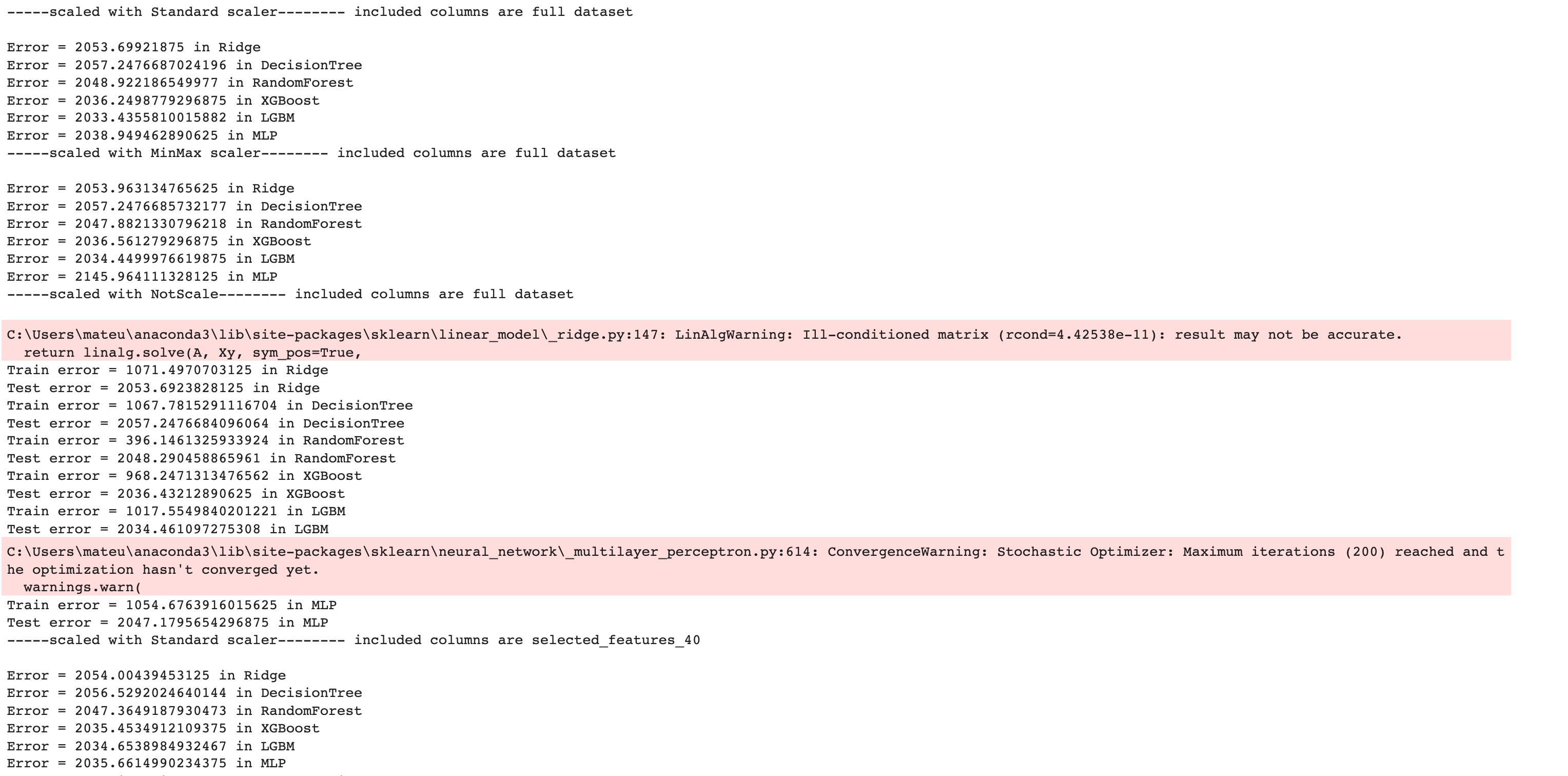
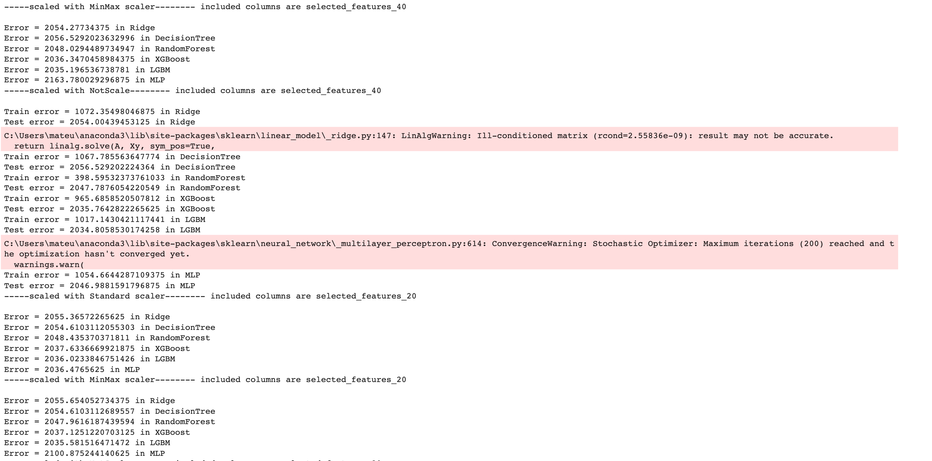
Now, we will use these structures more than once. That’s because most machine learning projects need these iterative processes to find the best performance model.

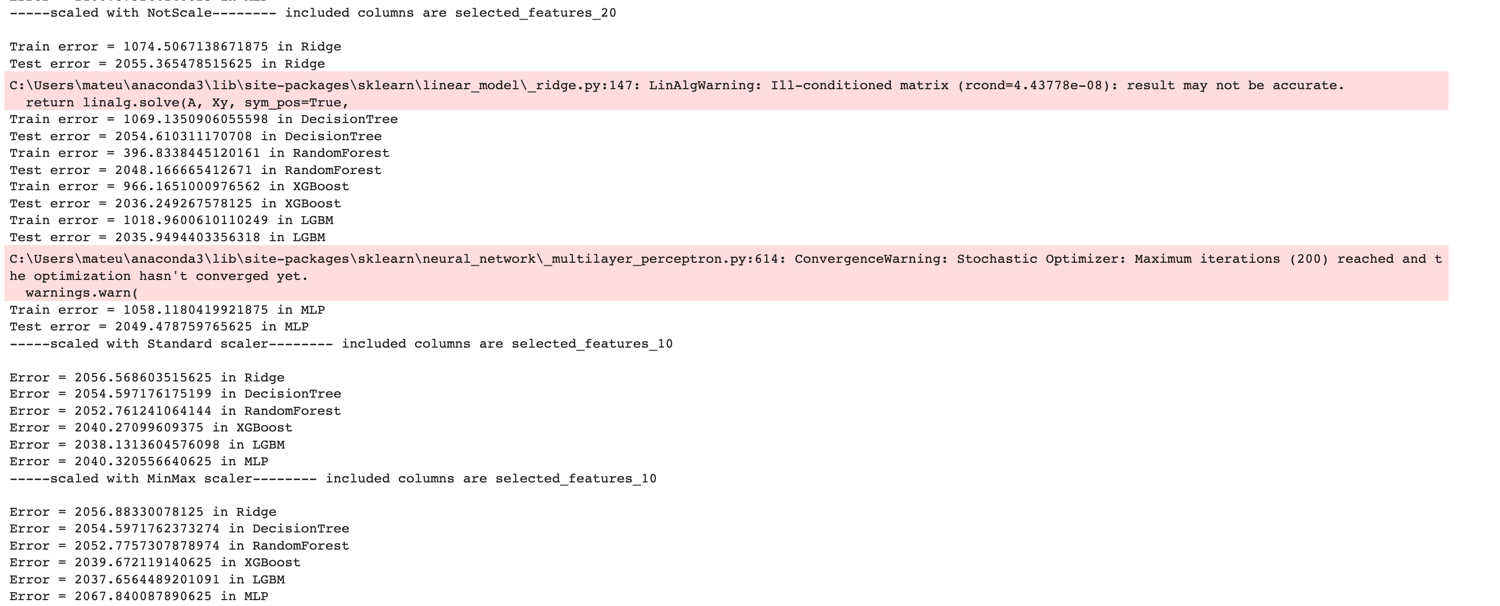
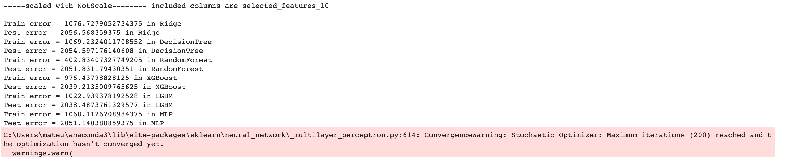
Here is the output of our code.

Now let’s create a DataFrame by using the pandas DataFrame() function to analyze our results further.

pred_df = pd.DataFrame(pred_dict)
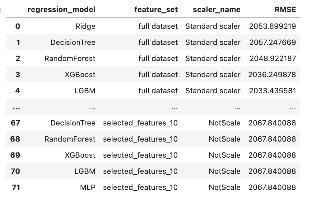
pred_df

Here is our output.

Plotting Results

Now, to see the results better, let’s visualize them.

pred_df.plot(kind='bar', figsize=(12,8))

Here is our graph containing the results.

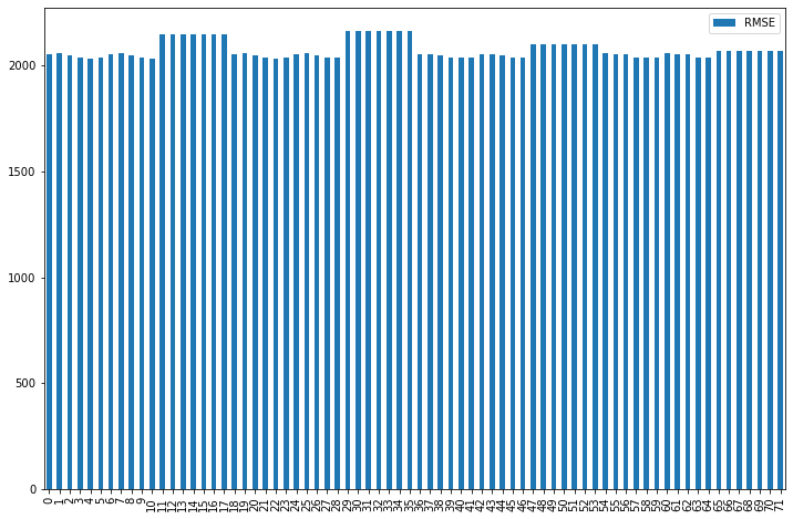
It looks like we have high errors in all our models. Also, the models tell us that not scaling made our model worse, so we will select one of our scalers. When we decrease the feature size, the model performance increases, but after 40, it continues decreasing, so we will select 40 features for our model.

Changing The Frame

There’s still room for improvement. Let’s change the problem a little bit by predicting prep duration first.

Then we will calculate "actual_total_delivery_duration” after the prediction.

To do that, we have to subtract store_to_consumer_driving_duration and order_to_place_duration from the actual_total_delivery_duration to find prep_duration_pred.

Prep_duration_pred= (actual total delivery duration) - (store to consumer driving duration) -(order to place duration).

After that, we will repeat the whole process, but we will select only 40 features and a standard scaler. So we will have 6 different predictions. Let’s see the code.

train_df["prep_time"] = train_df["actual_total_delivery_duration"] - train_df["estimated_store_to_consumer_driving_duration"] - train_df["estimated_order_place_duration"]

scalers = {
    "Standard scaler": StandardScaler(),
}

feature_sets = {
    "selected_features_40": importances.sort_values(by='Gini-importance')[-40:].index.tolist(),
}

for feature_set_name in feature_sets.keys():
    feature_set = feature_sets[feature_set_name]
    for scaler_name in scalers.keys():
        print(f"-----scaled with {scaler_name}-------- included columns are {feature_set_name}")
        print("")
        for model_name in regression_models.keys():  
            X = train_df[feature_set].drop(columns=["estimated_store_to_consumer_driving_duration", 
                                           "estimated_order_place_duration"])
            y = train_df["prep_time"]
       
            X_train, X_test, y_train, y_test = train_test_split(X, y, test_size=0.2, random_state=42)
            train_indices = X_train.index
            test_indices  = X_test.index
            
            
            X_scaled, y_scaled, X_scaler, y_scaler = scale(scalers[scaler_name], X, y)
            
            
            X_train_scaled, X_test_scaled, y_train_scaled, y_test_scaled = train_test_split(X_scaled, y_scaled, test_size=0.2, random_state=42)
            _, y_predict_scaled, _, _ = make_regression(X_train_scaled, y_train_scaled[:,0], X_test_scaled, y_test_scaled[:,0], regression_models[model_name], model_name, verbose=False)
            rmse_error, y_predict = rmse_with_inv_transform(y_scaler, y_test, y_predict_scaled, model_name)
            pred_dict["regression_model"].append(model_name)
            pred_dict["feature_set"].append(feature_set_name)
            pred_dict["scaler_name"].append(scaler_name)
            pred_dict["RMSE"].append(rmse_error)

Here is our output.

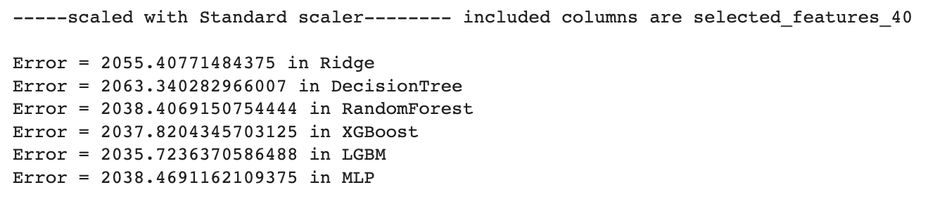
It looks like LGBM outperforms our remaining models every time so we will continue with that.

Here is the code.

# not scaling affects the performance, so continue to scale, but it doesn't matter much which scaler we used
scalers = {
    "Standard scaler": StandardScaler(),
}

feature_sets = {
    "selected_features_40": importances.sort_values(by='Gini-importance')[-40:].index.tolist(),
}

regression_models = {
    "LGBM": LGBMRegressor(),
}

for feature_set_name in feature_sets.keys():
    feature_set = feature_sets[feature_set_name]
    for scaler_name in scalers.keys():
        print(f"-----scaled with {scaler_name}-------- included columns are {feature_set_name}")
        print("")
        for model_name in regression_models.keys():  
            #drop estimated_store_to_consumer_driving_duration and estimated_order_place_duration
            X = train_df[feature_set].drop(columns=["estimated_store_to_consumer_driving_duration", 
                                           "estimated_order_place_duration"])
            y = train_df["prep_time"]
            
            
            X_train, X_test, y_train, y_test = train_test_split(X, y, test_size=0.2, random_state=42)
            train_indices = X_train.index
            test_indices  = X_test.index
            
            
            X_scaled, y_scaled, X_scaler, y_scaler = scale(scalers[scaler_name], X, y)
            
            
            X_train_scaled, X_test_scaled, y_train_scaled, y_test_scaled = train_test_split(X_scaled, y_scaled, test_size=0.2, random_state=42)
            _, y_predict_scaled, _, _ = make_regression(X_train_scaled, y_train_scaled[:,0], X_test_scaled, y_test_scaled[:,0], regression_models[model_name], model_name, verbose=False)
            rmse_error, y_predict = rmse_with_inv_transform(y_scaler, y_test, y_predict_scaled, model_name)
            pred_dict["regression_model"].append(model_name)
            pred_dict["feature_set"].append(feature_set_name)
            pred_dict["scaler_name"].append(scaler_name)
            pred_dict["RMSE"].append(rmse_error)

Here is our output.

Extract Predictions

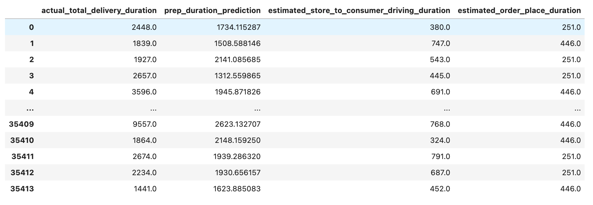
Now, let’s define a dictionary to choose the best-performance model and extract the prep_duration predictions.

It contains the actual_total_delivery_duration, estimated_store_to_consumer_driving_duration,  and estimated_order_place_duration by using our indices.

Then we will also add prep_duration_prediction by using y_pred.

pred_values_dict = {
    "actual_total_delivery_duration": train_df["actual_total_delivery_duration"][test_indices].values.tolist(), 
    "prep_duration_prediction":y_predict[:,0].tolist(),
    "estimated_store_to_consumer_driving_duration": train_df["estimated_store_to_consumer_driving_duration"][test_indices].values.tolist(),
    "estimated_order_place_duration": train_df["estimated_order_place_duration"][test_indices].values.tolist(),             
}

Now it’s time to convert that dictionary into a DataFrame. We will find sum_total_delivery_duration after this step.

We will also find an error by using the mean_squared_error() method. It needs an array to make the calculation.

values_df = pd.DataFrame.from_dict(pred_values_dict)
values_df

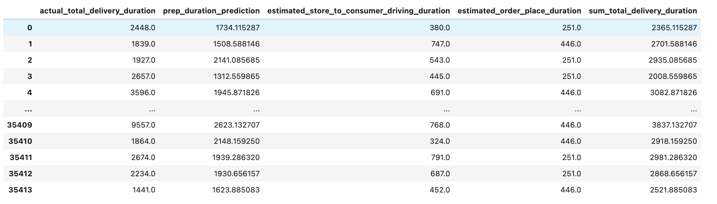
Since we already made this calculation earlier, we should turn this back by adding estimated_store_to_consumer_driving_duration and estimated_order_place_duration to prep_duration_prediction to find sum_total_delivery_duration. After that, let’s see our DataFrame.

values_df["sum_total_delivery_duration"] = values_df["prep_duration_prediction"] + values_df["estimated_store_to_consumer_driving_duration"] + values_df["estimated_order_place_duration"]
values_df

Let’s calculate the mean squared error.

mean_squared_error(values_df["actual_total_delivery_duration"], values_df["sum_total_delivery_duration"], squared=False)

Here is our output.

We still have a high level of errors. Let’s change the frame one last time. Here we will use prep_duration_prediction, estimated_store_to_consumer_driving_duration, and estimated_order_place_duration to predict actual_total delivery_duration. Do not forget to split your data again

X = values_df[["prep_duration_prediction", "estimated_store_to_consumer_driving_duration", "estimated_order_place_duration"]]
y = values_df["actual_total_delivery_duration"]
X_train, X_test, y_train, y_test = train_test_split(X, y, test_size=0.2, random_state=42)

Alright, now let’s apply the models.

regression_models = {
    "LinearReg" : linear_model.LinearRegression(),
    "Ridge" : linear_model.Ridge(),
    "DecisionTree" : tree.DecisionTreeRegressor(max_depth=6),
    "RandomForest" : RandomForestRegressor(),
    "XGBoost": XGBRegressor(),
    "LGBM": LGBMRegressor(),
    "MLP":  MLPRegressor(),
}
for model_name in regression_models.keys():
    _, y_predict, _, _= make_regression(
        X_train, y_train, X_test, y_test,regression_models[model_name], model_name, verbose=False)
    print("RMSE of:",model_name, mean_squared_error(y_test,y_predict, squared=False))

Here is our output.

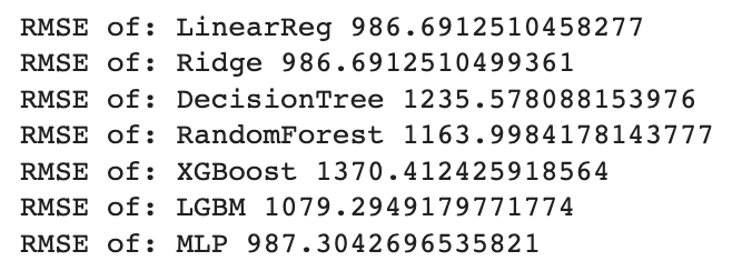
As we can see from the output, our error rate drops by nearly half. This model’s performance is better than our other results. So, that may be our solution.

Deep Learning

Now, as a final step, let’s find out if we would have better results by using a neural network. Let’s create a function using both Keras and TensorFlow to build a model that can predict the actual total delivery time. Our model will be a sequential model with dense layers, using the relu and linear activation functions. We will use the Stochastic Gradient Descent optimizer and the Mean Squared Error loss function, and we will also calculate the root mean squared error.

import keras
from keras.models import Sequential
from keras.layers import Dense
import tensorflow as tf
tf.random.set_seed(42)

def create_model(feature_set_size):
    
    model = Sequential()
    model.add(Dense(16, input_dim=feature_set_size, activation='relu'))
    model.add(Dense(1, activation='linear'))
    

    model.compile(optimizer='sgd', loss='mse',
        metrics=[tf.keras.metrics.RootMeanSquaredError()])
    
    return model

Now we will call our function.

print(f"-----scaled with {scaler_name}-------- included columns are {feature_set_name}")
print("")
model_name = "ANN"   
scaler_name = "Standard scaler"
X = values_df[["prep_duration_prediction", "estimated_store_to_consumer_driving_duration", "estimated_order_place_duration"]]
y = values_df["actual_total_delivery_duration"]
X_train, X_test, y_train, y_test = train_test_split(X, y, test_size=0.2, random_state=42)
X_scaled, y_scaled, X_scaler, y_scaler = scale(scalers[scaler_name], X, y)
X_train_scaled, X_test_scaled, y_train_scaled, y_test_scaled = train_test_split(
    X_scaled, y_scaled, test_size=0.2, random_state=42)
print("feature_set_size:",X_train_scaled.shape[1])
model = create_model(feature_set_size=X_train_scaled.shape[1])
history = model.fit(X_train_scaled, y_train_scaled, epochs=100, batch_size=64, verbose=1)
y_pred = model.predict(X_test_scaled)
rmse_error = rmse_with_inv_transform(y_scaler, y_test, y_pred, model_name)
pred_dict["regression_model"].append(model_name)
pred_dict["feature_set"].append(feature_set_name)
pred_dict["scaler_name"].append(scaler_name)
pred_dict["RMSE"].append(rmse_error)

Here is the result.

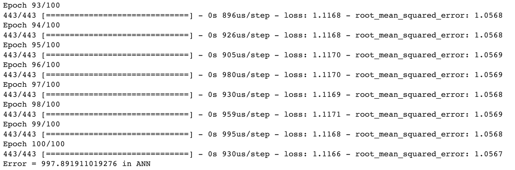
Now, the error level is not much different than our machine learning models.

Let’s draw a graph to show the relationship between the epoch and loss. Also, an epoch refers to one cycle through the entire data frame, and the loss measures the differences between the actual values and the predicted ones across the entire data frame.

Here is the code.

plt.plot(history.history['loss']) 
plt.title('Model loss') 
plt.ylabel('Loss') 
plt.xlabel('Epoch') 
plt.show()

And this is the output.

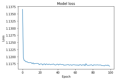
Based on these results, it seems that linear regression and LGBM will be our best solutions. Yet we could potentially achieve better results by fine-tuning the hyperparameters with various methods. However, considering the time and effort involved, this model is also promising and efficient.

Conclusion

In this data project, the goal was to predict the total delivery duration of food orders placed on DoorDash, a company for ordering food online and delivering it to the customers’ location.

Timely delivery is important for both customers and businesses. By accurately predicting delivery times, DoorDash can improve customer satisfaction. We divided the problem into four sections. We discussed data preparation and modeling in the first section, including feature creation and engineering. Then, we removed redundant and collinear features in section two by using a heatmap.

In section three, we checked multicollinearity by using the VIF score, and then we did feature selection with PCA and Gini’s index.

Finally, we created both Machine Learning and Deep Learning models in the last section.

In the Machine Learning section, we applied 6 different regression algorithms on 4 different feature sets with 3 different scalers, so we got 72 results. Also, we reframed the problem many times by changing the predictors and predicted values. After that, we built a neural net by using the sequential model with dense layers and many other parameters to optimize our model.

If you are a beginner, check out these top 19 data science project ideas. Also, If you liked this Data project, there are many others on our platform. See you there!