Creating R Programming Histogram for Data Visualization

Step-by-step guide to creating, customizing, and interpreting R programming histograms using real student performance data

Most data reports begin with simple visualizations, and histograms are a great way of visualizing your data because they show how data points are distributed in your dataset. This helps you detect clusters, gaps, or even outliers before any advanced analysis or modeling begins.

In this article, we will explore R programming histograms, learn how to create and adjust them, and apply them to a real-world dataset. Let’s get started!

What Is a Histogram in R Programming?

A histogram is a type of bar plot that maps how data points fall into ranges. Each bar represents a group of values (called a bin).

Histograms display the distribution of continuous data. You see the general pattern rather than examining each value separately.

If you're also working in Python, you might want to check out how to create a Matplotlib histogram for a side-by-side comparison with R.

When Should an R Programming Histogram Be Used?

Histograms can be used to determine the distribution of numerical data. You can use it to:

• Check data distribution
• Spot outliers and gaps
• Compare data before and after filtering

No other charts give you that much information at first look, and that’s why it is often used as a first step in data exploration.

Basic Syntax of Histogram in R Programming

You can use the hist() function in R. It’s a built-in function that can run with just one argument. It takes your numerical values and breaks them into bins, drawing bars to show how these values are spread. Let’s create a mock-up dataset and visualize it.

Step 1: Sample Data

Let’s create some sample student score data.

set.seed(123)
student_scores <- round(rnorm(100, mean = 70, sd = 10), 0)
head(student_scores)

Here is the output.

The data sample suggests that student scores fall between 60 and 90. However, since these are only the first rows, there may be additional student scores. Let's visualize the data to see.

Step 2: Visualize the Data

To visualize it all, we use the built-in function. Here is the code.

hist(student_scores)

Here is the output.

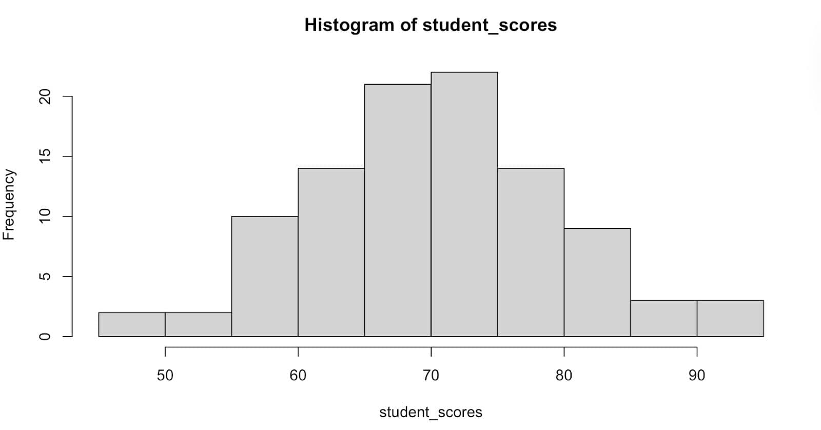
As you can see from the graph above, the distribution of student scores is evident, showing a range from 40 to 100.

How to Customize an R Programming Histogram for Better Insights

Although the default histogram is good, customization would be preferable. Let's examine how to enhance the aesthetics and educational value of your histogram step by step.

Step 1: Bins

Adjusting the number of bins alters how your data is distributed. Let’s adjust bins to discover.

hist(student_scores, breaks = 20)

This increases the number of bars by splitting your data into 20 intervals. Here is the output.

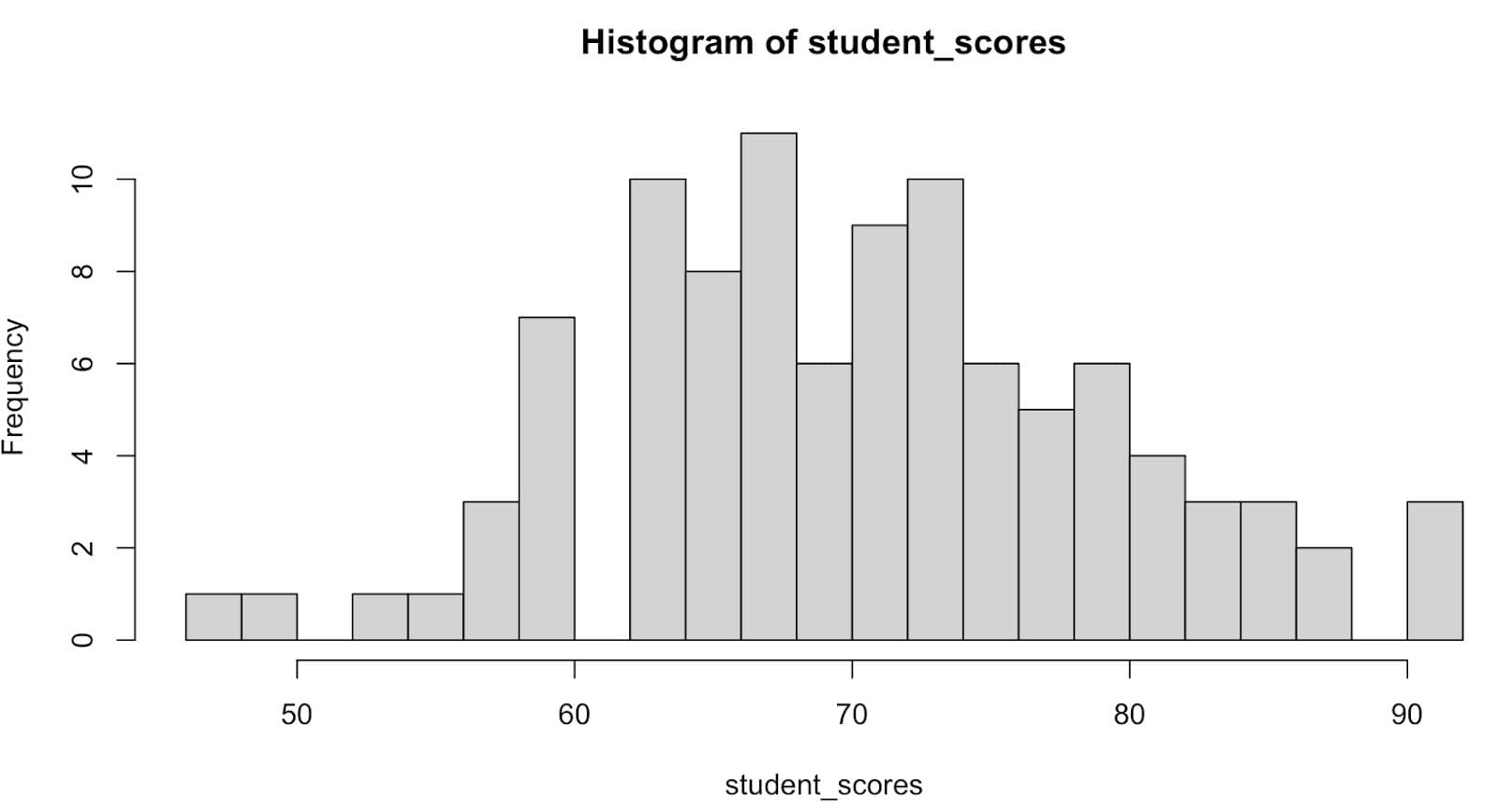
As you can see, there are gaps! So let’s switch back to 15.

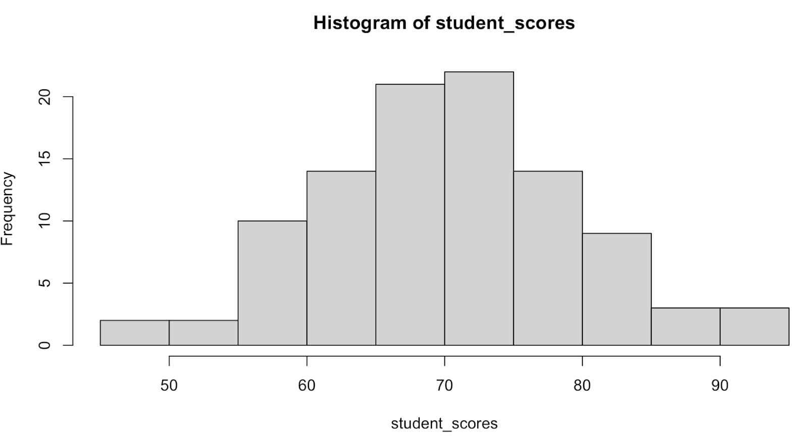
This looks better, but it’s the same graph we first created.

How does R choose the breaks? If you omit the breaks argument, hist will set them automatically based on the distributions of your dataset.

Step 2: Colors

Adding colors is straightforward and makes your graph more appealing.

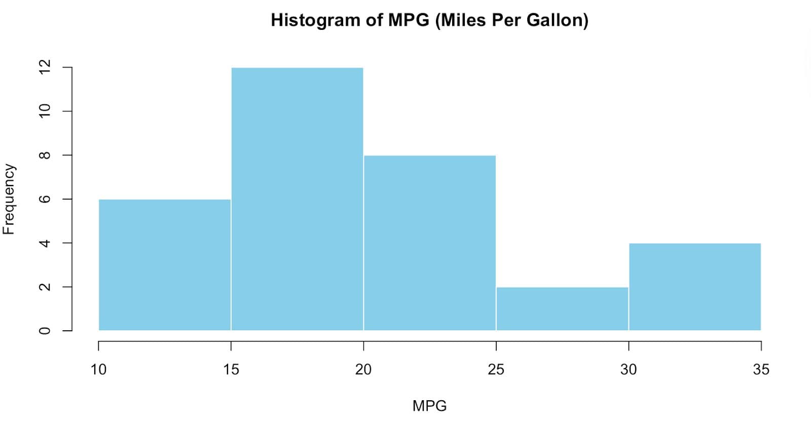
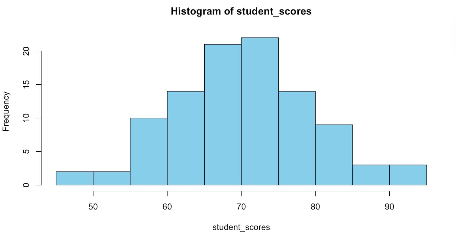
hist(student_scores, breaks = 15, col = "skyblue")

Here is the output.

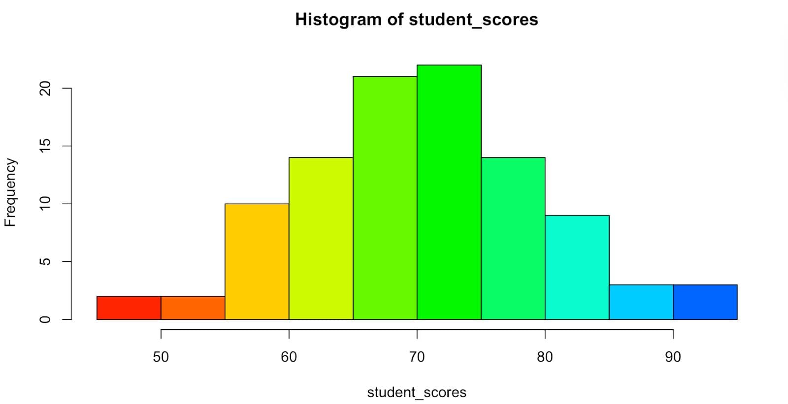
Instead of adding constant colors, you can also add gradients.

# Gradient color histogram
hist(student_scores,
     breaks = 15,
     col = rainbow(15))

Here is the output.

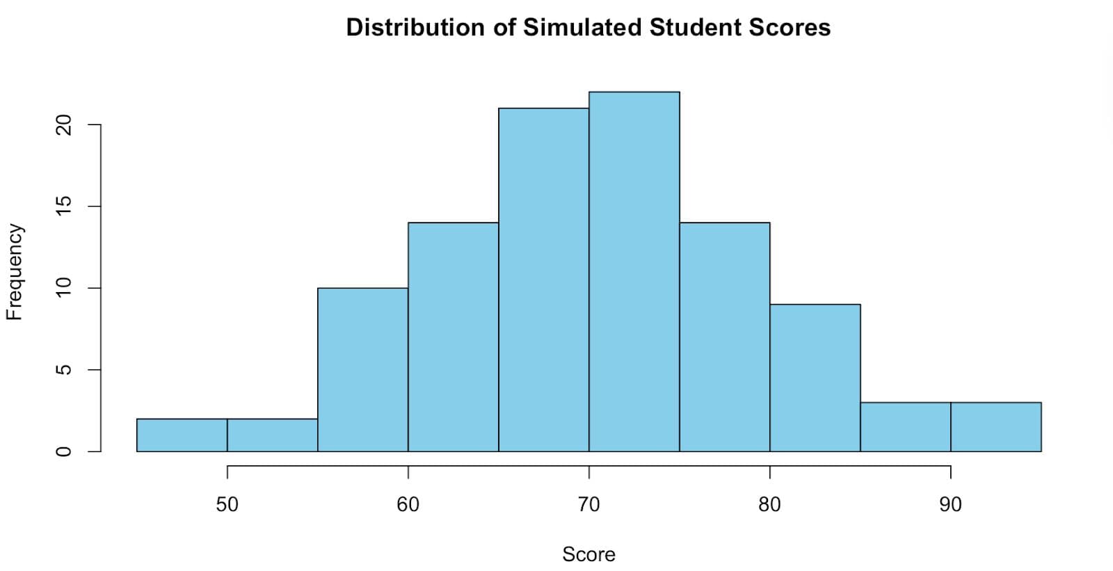
Step 3: Title and Axis Labels

Titles and axis labels can be adjusted. Let’s do that and see what the graph would look like.

hist(student_scores,
     breaks = 15,
     col = "skyblue",
     main = "Distribution of Simulated Student Scores",
     xlab = "Score",
     ylab = "Frequency")

Here is the output.

Real-World Use Case: R Programming Histogram for Student Performance Analysis

At this step, let’s use a dataset from the real world. In this data project, the goal is to analyze student achievement in Mathematics and Portuguese language, based on the data from two Portuguese schools.

Link to this data project: https://platform.stratascratch.com/data-projects/student-performance-analysis

Let’s take a look at the first few rows.

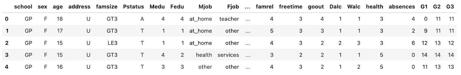
Here are the dataset columns.

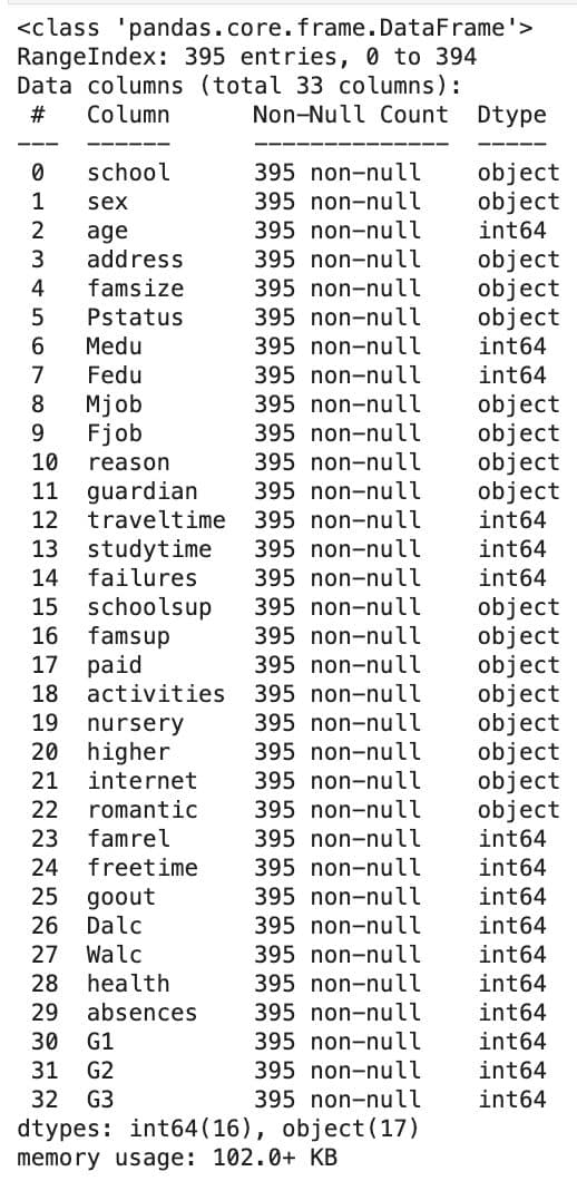
As you can see, there are 30+ columns, including School, sex, age, address, famsize, pstatus, and more.

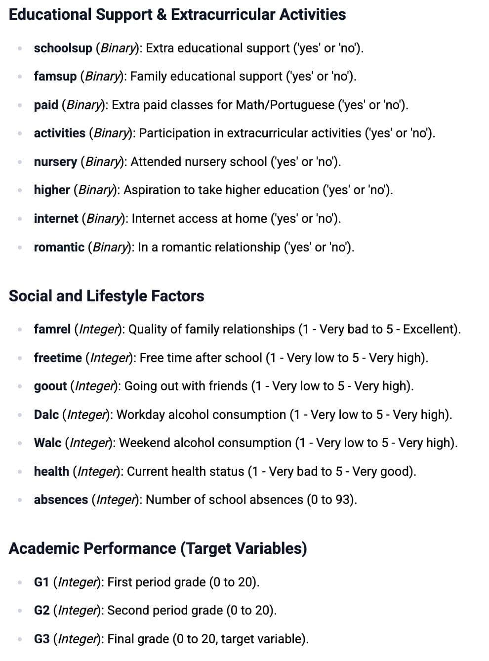
Let’s see the data dictionary.

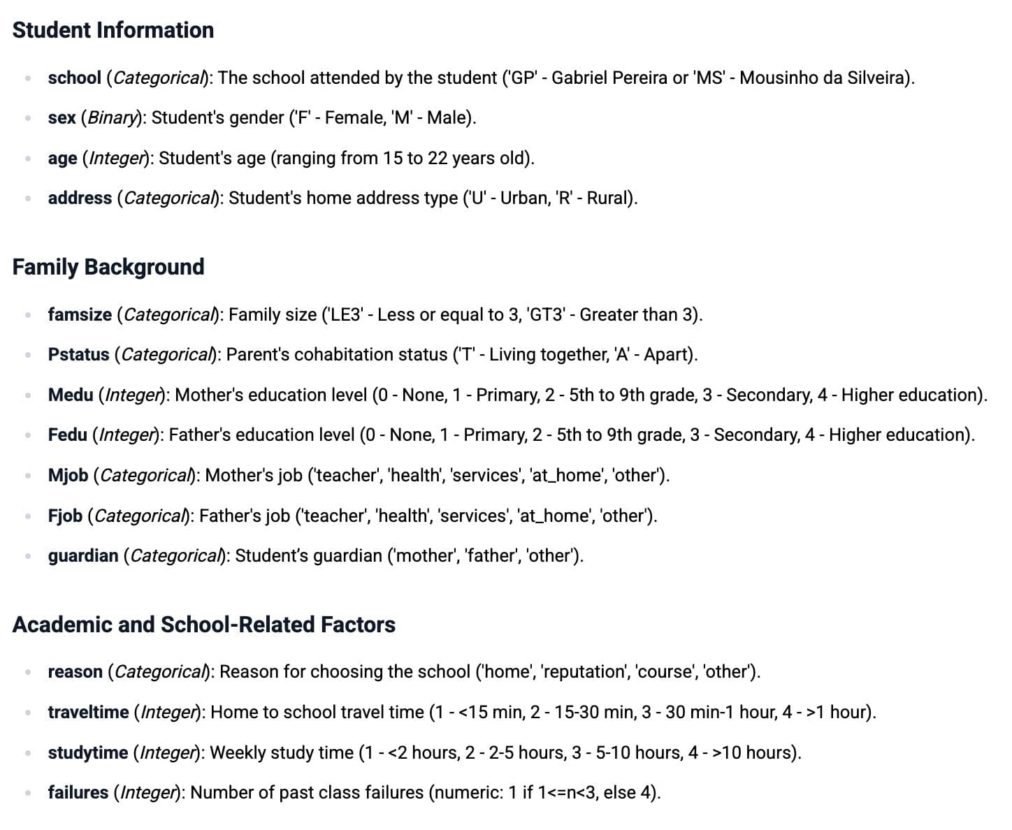
But there are more columns. Here are the rest of them with explanations.

Basic Histogram of Final Grades

Before customizing anything, let’s create a simple histogram using G3, the final grade.

hist(student_data$G3,
     main = "Distribution of Final Math Grades (G3)",
     xlab = "Final Grade",
     ylab = "Number of Students",
     col = "lightblue")

Here is the output.

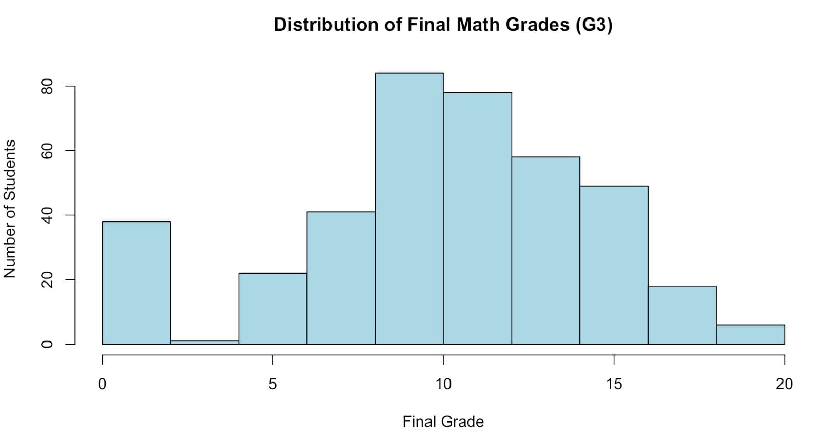
As seen in the chart above, the distribution of grades is centered around 10-12, with most students scoring between 5 and 15.

Custom Bins and Gradient Color

Next, let’s create a visual by controlling how grades are grouped and adding color dynamics.

Here is the code.

hist(student_data$G3,
     col = rainbow(10),
     main = "Final Math Grades (G3) with Gradient",
     xlab = "Grade",
     ylab = "Student Count")

Here is the output.

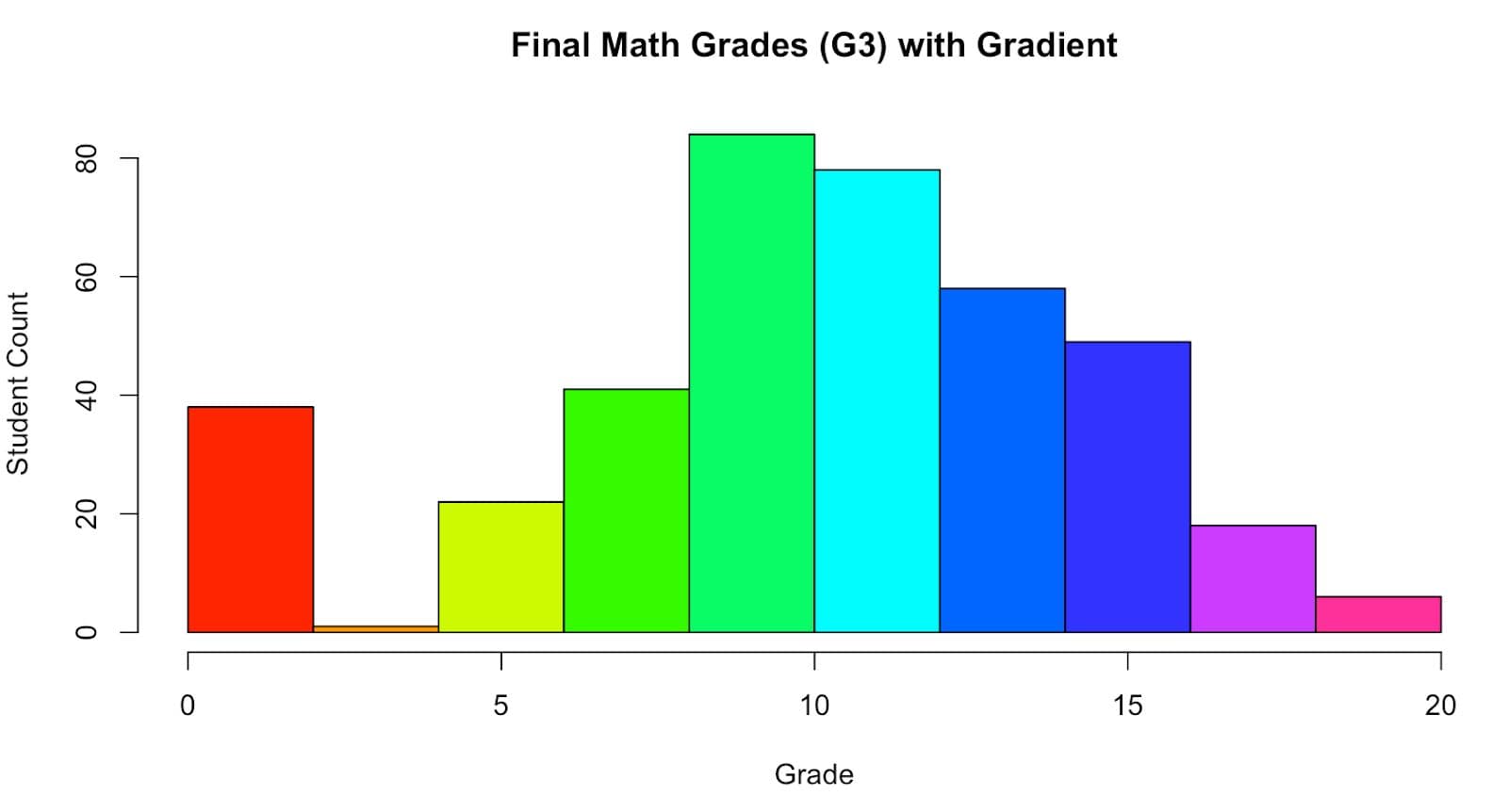
In this code, we add different colors for each bin by applying a rainbow color palette to enhance the contrasts. This makes it easier for viewers to distinguish grade clusters.

Compare Grade Distribution by Study Time

Let’s move beyond simple analysis and see how study time affects final grades. To do that, we can use ggplot2. In the code below, we will use ggplot2 to draw a graph of the final grade distribution (G3), across different levels of weekly study time by using color-coded histogram bars.

We map G3 to the x-axis and study the time to fill aesthetic to compare how each study-time group performs.

Here is the code.

library(ggplot2)
ggplot(student_data, aes(x = G3, fill = factor(studytime))) +
  geom_histogram(binwidth = 1, position = "identity", alpha = 0.5) +
  labs(title = "Grade Distribution by Study Time",
       x = "Final Grade (G3)",
       y = "Count",
       fill = "Study Time Level") +
  theme_minimal()

Here is the output.

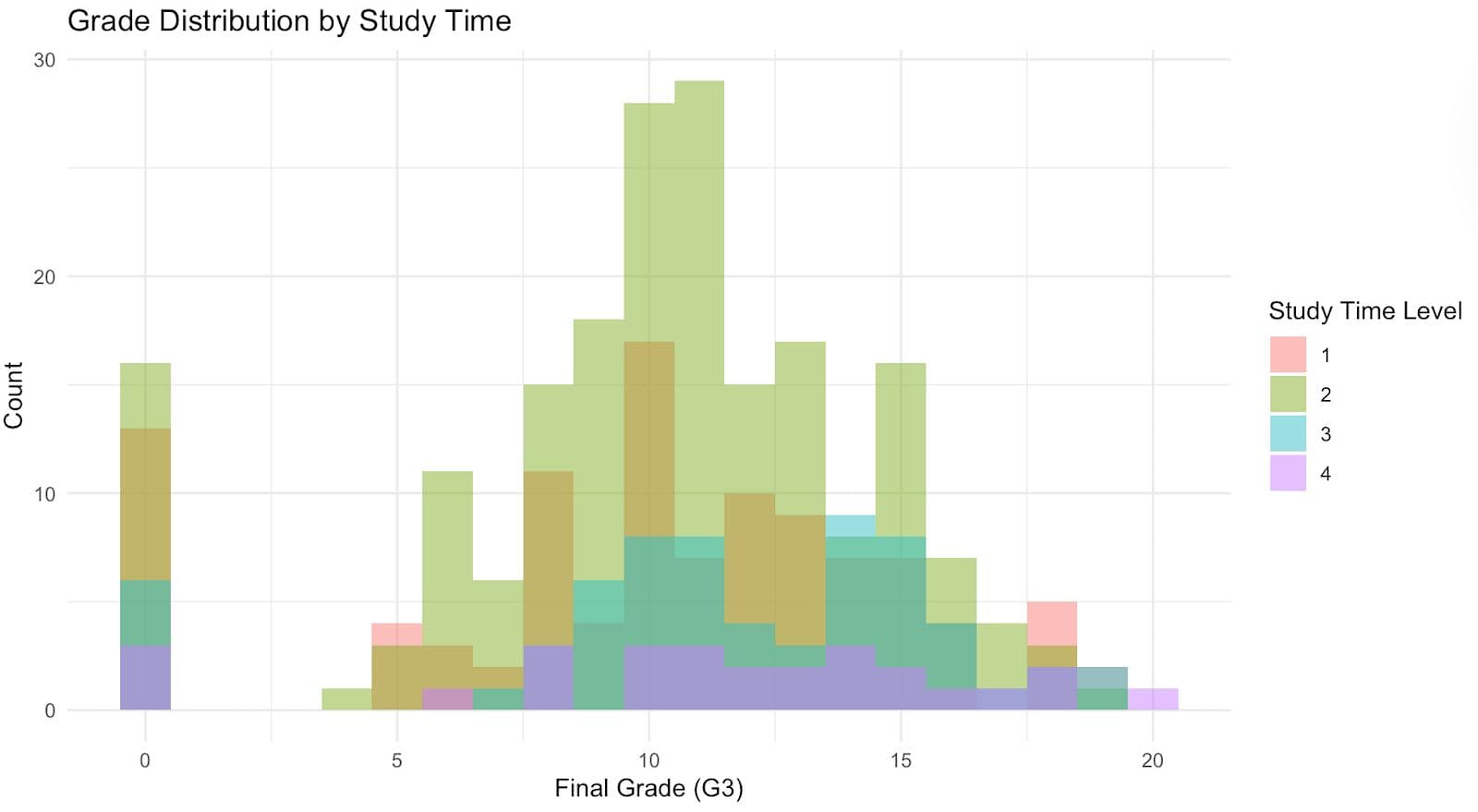
Here, each color represents a different study time level. You will notice that students with longer study time, level 4, tend to shift slightly toward the right, suggesting better performance.

Final Grade Distribution by Failure History

Now let’s answer this question;

Does a student’s history of class failures correlate with current academic performance?

A “failure” variable in the dataset indicates the frequency of a student's past course failures and how this may affect their final grade. In the code below, we use ggplot2 to visualize how grades are distributed based on students' past failure counts, using overlapping histograms grouped by failure history.

library(ggplot2)
ggplot(student_data, aes(x = G3, fill = factor(failures))) +
  geom_histogram(binwidth = 1, position = "identity", alpha = 0.5) +
  labs(title = "Final Grade Distribution by Failure History",
       x = "Final Grade (G3)",
       y = "Count",
       fill = "Number of Past Failures") +
  theme_minimal()

Here is the graph.

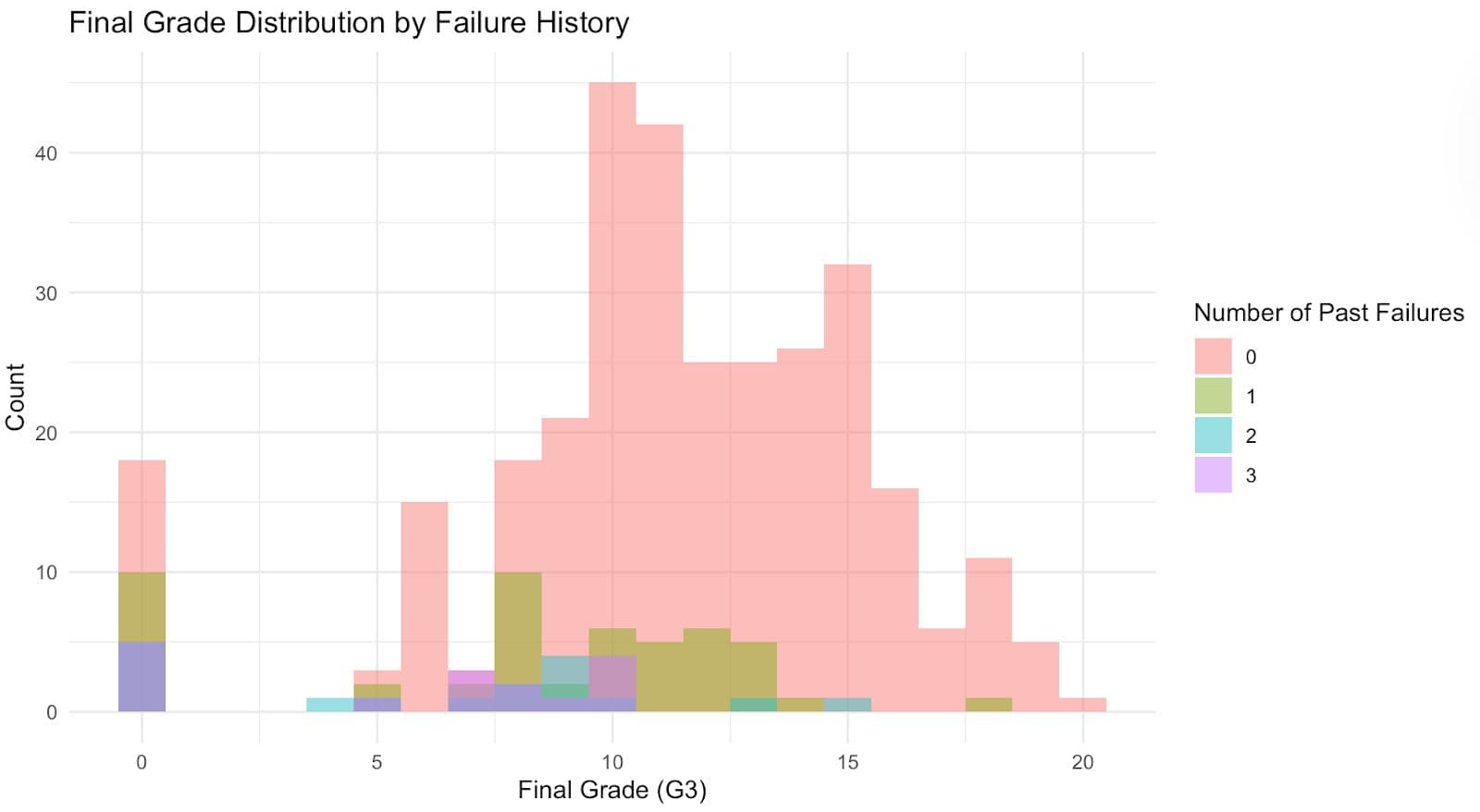
As you can see in the histogram:

• Students who perform well typically appear on the right side of the graph and have never failed before.
• One or more failures usually place a student in the lower half of the class, which translates into lower grades.
• Grade zones below 10 will have a noticeable presence, especially with the 2-3 failures.

This tells us that students who struggled before tend to continue struggling.

Final Thoughts

In this article, we have explored how histograms can be created by using R and how they can be customized. Then, we used a real-life dataset to answer questions to find a correlation between students' success and other factors like the number of past failures or study time level.

With just a few lines of code, an R programming histogram can reveal patterns that might otherwise go unnoticed. It's one of the simplest yet most powerful tools for initial data exploration.