8 Python Libraries For Math, Data Analysis, ML, and DL

Python Libraries for Math, Data Analysis, Machine Learning, and Deep Learning

What Are Python Libraries?

A Python library consists of pre-defined custom functions that help write neat and shorter scripts while doing tasks like data visualization, data analysis, machine learning, or deep learning. Many different Python libraries exist in the community, and they all help data scientists with various tasks.If you wonder what library does what job, here’s an overview of 18 Python libraries every data scientist should know.

We already showed you how to work with the four data collection libraries.

It’s time to do the same with Python libraries you can use for maths, data analysis, machine learning, and deep learning.

Python Libraries for Math and Data Analysis

In data science, math, and data analysis play a vital role in the process of converting raw data into actionable insights.

They include applying mathematical operations to the data to uncover patterns, trends, and relationships.

The main goal is to transform unstructured data into a structured format that can be analyzed and used to make data-driven decisions.

After collecting data, data scientists use mathematical methods to perform, for example, feature engineering, which involves creating new variables from existing data to help improve the accuracy of predictive models.

Another example is to change your variables by applying mathematical operations to create linear regression between response and explanatory variables, like logarithms, square roots, polynomials, or more.

Data visualization is also an important aspect of math and data analysis in data science. It helps to identify trends and patterns in the data quickly and allows data scientists to communicate their findings in a clear and concise way.

In this article, we will mention pandas, known for data analysis and manipulation, but also includes some data visualization tools, which we will discover together.

Ultimately, the goal of math and data analysis in data science is to build predictive models that can accurately predict future events.

By using mathematical methods and algorithms, data scientists can train machine learning and deep learning models to make predictions based on historical data.

Before diving into machine learning and deep learning libraries, let’s mention 4 of these math and data analysis libraries, which will help you to transform this unstructured data into the unstructured version, in which you can apply machine learning and deep learning models.

4 Python Libraries for Math and Data Analysis Every Data Scientist Should Know

NumPy

Python's NumPy library is specifically designed for numerical data manipulation.

This library offers assistance for managing extensive arrays and matrices that possess multiple dimensions, along with mathematical functions to manipulate these arrays.

Let’s demonstrate this in an example.

First, import NumPy.

import numpy as np

After that, we will create a 3x3 matrix using an array function with NumPy.

# Create a 3x3 matrix
A = np.array([[1, 2, 3], [4, 5, 6], [7, 8, 9]])

Then we will calculate transpose by using numpyndarray.T property from NumPy.

# Transpose the matrix
A_transposed = A.T

After that, we will multiply the matrices A and A_transposed by using the @ operator.

# Multiply the matrices
C = A @ A_transposed

This operator is used to perform matrix multiplication in NumPy.

The result is then assigned to c and printed to see the result.

# Print the result
print(C)

Here is the output.

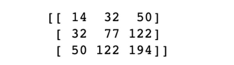
NumPy Python Library for Math and Data Analysis

As a result, this code transposes the matrix, multiplies it with the original matrix, and prints the result.

SciPy

This library is utilized for scientific computation in the Python programming language.

Similarly, it furnishes capabilities to operate on arrays, optimize numerical data, and process images and signals, among other features.

Here’s an example. First, import the library.

import scipy.linalg as la

Then we will define the coefficients of the linear system:

a – 3x3 array that represents the coefficients of the three equations in the system.
b – contains the constant terms of the equations in the system.

# Define the coefficients of the linear system
a = np.array([[1, 2, 3], [4, 5, 6], [7, 8, 9]]) #
b = np.array([1, 2, 3])

Then the solve() function is defined to solve the system of equations, and we print the result.

# Solve the linear system
x = la.solve(a, b)

# Print the solution
print(x)

Here is the result.

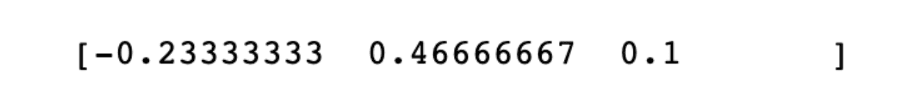
The code we showed solves the system of linear equations defined by a and b arrays and prints the solution vector to the screen.

math

math is a built-in library in Python that provides access to mathematical functions.

It includes functions for basic math operations, trigonometry, logarithms, and more.

It is generally used for mathematical operations that are not covered by NumPy or SciPy.

Let's look at the code syntax.

Import the math library.

import math

After that, we will compute the square root of 256 by using the sqrt function in the math library, and we also store the result in the x variable.

import math
# compute the square root of 256
x = math.sqrt(256))

After that, the assert statement is used to check if the code is true by equaling it to 16.

If the code continues to run, but the result is not actually the square root of 256, then it will raise an error.

Yet the square root of 256 is 16.

So our code prints "Code works just fine, x is equal to 16."

assert x == 16
print("Code works just fine, x is equal to 16")

Here is our output.

What if we use false conditions?

Here is an example of it.

We first compute sin(0) and assign the result to y.

import math
# compute sin 0
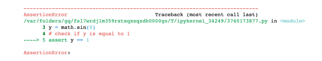
y = math.sin(0)

Sin(0) is actually 0, yet to see how the assert works, we write assert with a false condition, which is y = 1.

# check if y is equal to 1
assert y == 1

Here is the output. It throws an assertation error because y has to be 0.

pandas

Pandas is a powerful open-source Python library for data analysis and data visualization.

It provides powerful data structures, like DataFrame, and built-in functions that make it easy to work with and manipulate data.

Pandas can be used to perform mathematical calculations, such as statistics and linear algebra, as well as more advanced data analysis techniques, such as machine learning and deep learning.

Pandas can also be used to create data visualizations, such as plots and charts, to help visualize and explore your data.

Now let’s look deeper into by looking at panda's syntax.

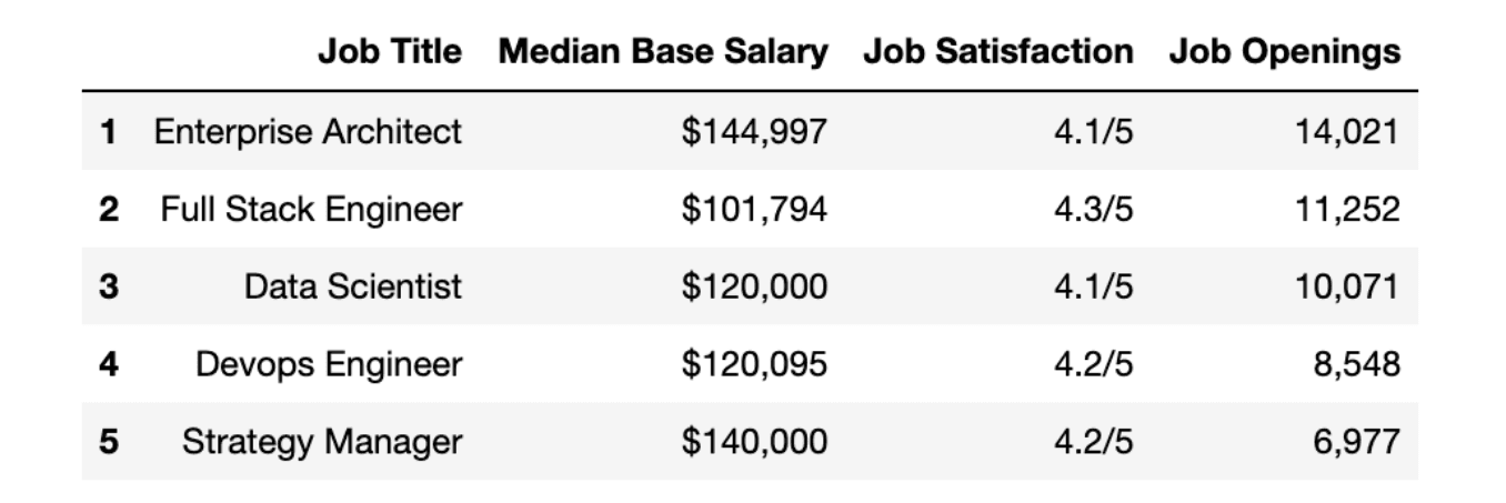
Here we have a data frame from Glassdoor.

Glassdoor has created a list of 50 Best Jobs in America, considering factors such as median salary, job satisfaction, and job openings.

This list is based on Glassdoor's unique and extensive data on employment, salaries, and companies.

Now, let's glance at our data frame using the head() method.

Here is the code.

# check our data frame
df.head()

Here is the output.

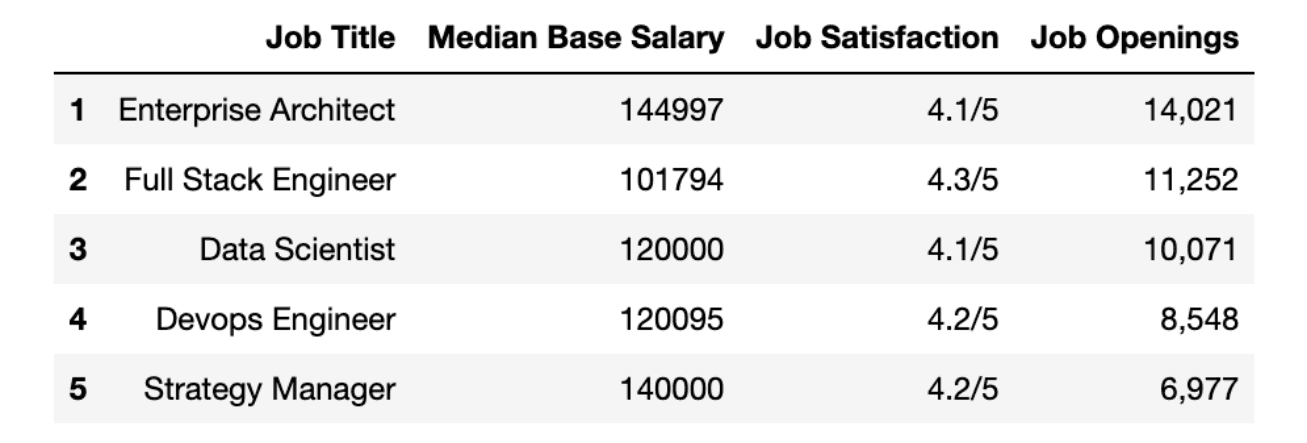
Pandas Python Library for Math and Data Analysis

Alright, to do further analysis, we should remove the dollar sign using the replace() method.

Here is the code.

# remove the dollar sign
df["Median Base Salary"] = df["Median Base Salary"].str.replace("$", "")

Also, let's remove the comma by using the str method with the replace() method. Then we will turn this type into an integer to do an analysis.

Here is the code.

# check if y is equal to 1
fifty_best["Median Base Salary"] = fifty_best["Median Base Salary"].str.replace(",", "").astype(int)

Now, let’s see our data frame again.

# check the first five rows.
df.head(5)

Here is the output.

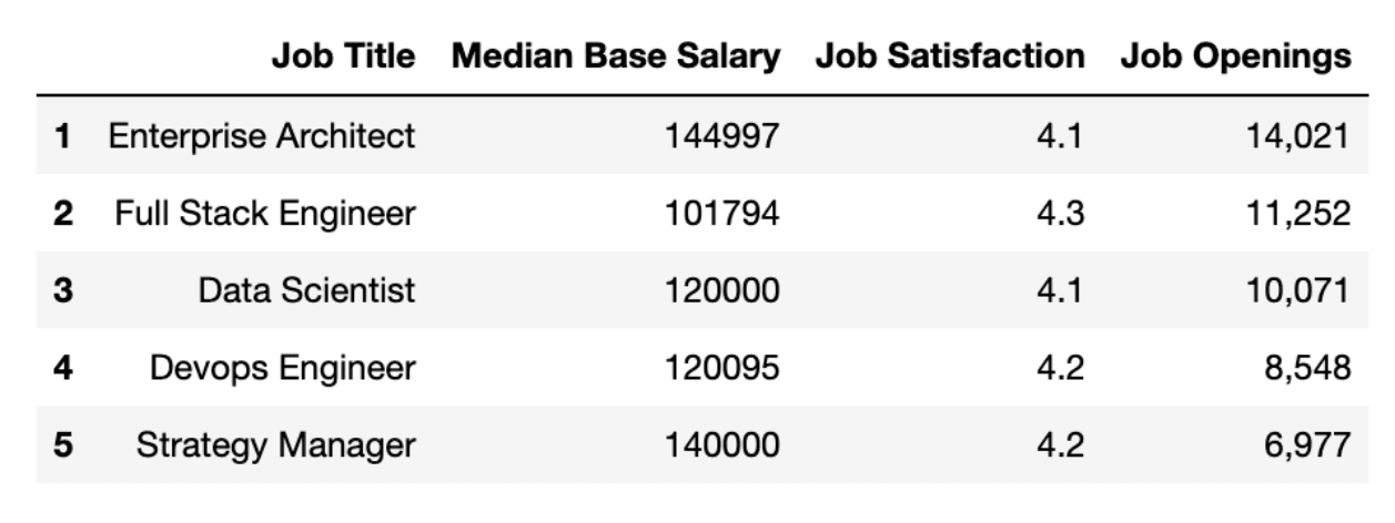
Now we have issues with our Job Satisfaction column. We must remove the string after ‘/’ so we can use this column.

We will again use the str method. This time, we’ll use it with the split() method, select the first element of str, and turn the type into float.

Here is the code.

# format the job satisfaction column.
df["Job Satisfaction"] = df["Job Satisfaction"].str.split("/").str[0].astype(float)

Let's see our data frame again.

# check first rows of our data frame
df.head(5)

Here is the output.

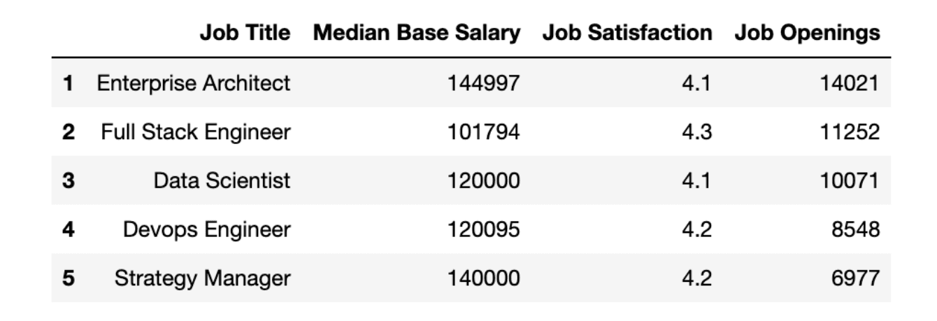
As a final step, we should remove the comma from the Job Openings columns. Additionally, we will change the data type to an integer to do further analysis.

# format the Job Openings column.
df["Job Openings"] = df["Job Openings"].str.replace(",", "").astype(int)

Now, let’s check our data frame again.

# check first rows of our data frame
df.head(5)

Here is the output.

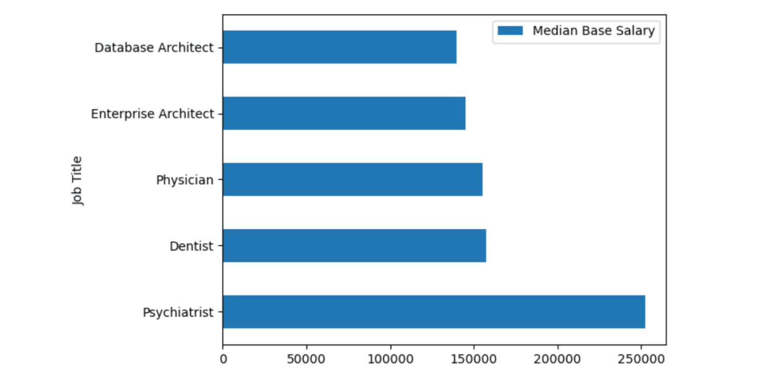
Now, let's find the 5 jobs that have the highest salary. We will use pandas data analysis features among data visualization features. First, we will sort values by salary and select the first 5 jobs using the head() method.

Then we will use .plot.barh method to draw horizontal bar graphs by selecting Job Title as x and Salary as y-axis.

Let's see our code.

# barplot with pandas
df.sort_values(by = "Median Base Salary", ascending = False).head(5).plot.barh(x = "Job Title", y = "Median Base Salary")

Here is the output.

Now it’s time to add multiple conditions. Salary should not be the only condition when choosing a profession, right?

Let's define basic requirements as follows;

Job Satisfaction - 4.0
Job Openings - 7,500
Base Salary - 10,0000

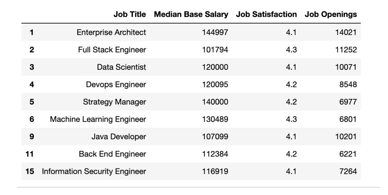
We will filter data by applying index slicing.

# filtering to find best jobs
best_jobs  = df[(fifty_best["Job Satisfaction"] > 4) 
           & (df["Median Base Salary"] > 100000) 
           & (df["Job Openings"] > 5000)]

Now, let's see best jobs as a data frame first.

Here is the code.

best_jobs

Here is the output.

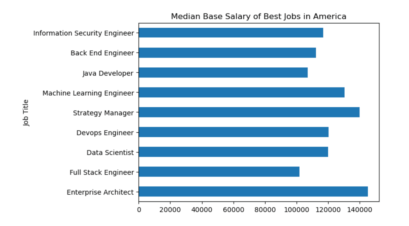
By now, we are familiar with drawing graphs in pandas. We will now use the matplotlib library with pandas to add a title.

Here is the code.

# let's draw a graph.
import matplotlib.pyplot as plt
best_jobs.plot.barh(x = "Job Title", y = "Median Base Salary")
plt.title("Median Base Salary of Best Jobs in America")
plt.legend().remove()
plt.show()

Here is the output.

Python Libraries for Machine Learning and Deep Learning

Machine learning is a type of AI that allows users and industries to come up with more accurate predictions.

It is founded on the concept that programs can assimilate knowledge from data, recognize patterns, and take decisions with minimal human involvement.

Deep learning is a sub-field of machine learning that uses algorithms such as neural networks to learn and make predictions. They can handle large and complex data sets. Some well-known examples include face recognition, and speech recognition, and even the Netflix recommendation system uses the same technology.

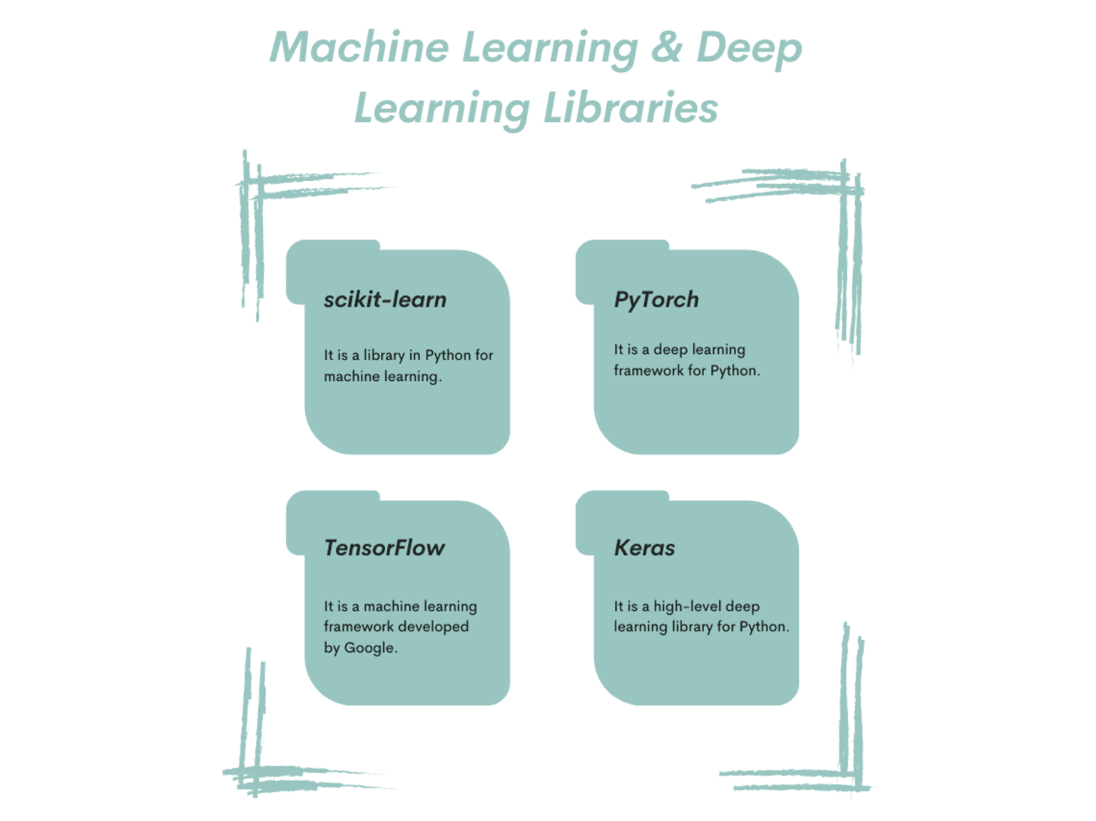
scikit-learn

Scikit-learn is a well-known machine learning library in Python, offering a vast array of tools to construct and assess machine learning models.

It was developed by a team of researchers from INRIA, which is a French institute for computer science and applied mathematics. The lead developer of it is Fabian Pedregosa.

Built on NumPy, SciPy, and Matplotlib, it is intended to enhance the readability, comprehensibility, and efficiency of machine learning code.

scikit-learn has many different algorithms for classification, regression, and clustering. Also, it has many features to enhance your model efficiencies, like dimension reduction, model selection, or preprocessing.

Let's dive into the coding problem to see the syntax of this library.

In the example, we’ll use scikit-learn to train a logistic regression model to classify iris flowers according to their petal and sepal lengths.

First, let's import datasets to use the Iris data set for this problem.

from sklearn import datasets
from sklearn.model_selection import train_test_split
from sklearn.linear_model import LogisticRegression

Now, we have to load data.

# Load the iris dataset
iris = datasets.load_iris()

The train_test_split function is used to split the data set into train and test. This helps us to evaluate the algorithm in the data that it has not seen before.

# Split the dataset into train and test sets
x_train, x_test, y_train, y_test = train_test_split(iris.data, iris.target, random_state=0)

After that, first, we will define the algorithm, which will be logistic regression.

# Define Model
model = LogisticRegression()

The logistic regression algorithm is often used in classification problems.

Okay, now we will use the fit() function to train the model.

# Train a logistic regression model on the training data
model.fit(x_train, y_train)

As a final step, we will evaluate our model by using the score() function on the test data.

This function returns the model's accuracy, which is the percentage of correct predictions made on the test set. By using this function in the round() function with 2 as an argument, we will see the output with 2 decimals.

Here’s the code.

# Evaluate the model on the test data
print(round(model.score(x_test, y_test),2))

Here is the output.

scikit-learn Python Library for Machine Learning and Deep Learning

As we can see, the accuracy is 0.97, which is pretty good.

Keras

Keras is a Python-based open-source framework used for deep learning, constructed atop TensorFlow.

It provides high-level API that makes it easy to define and train deep learning models and includes support for Convolutional Neural Networks(CNN) and Recurrent Neural Networks(RNN), which are popular network architectures.

CNN is often used in Computer Vision, Natural Language Processing, and RNN is often used in Speech Recognition, Natural Language Processing, and more.

Keras was released in 2015 and developed by François Chollet, a software engineer at Google.

To show you how it works, we will aim to predict IMDB review, also known as sentiment analysis.

The main purpose is to predict whether the IMDB review is positive or negative.

This model will take a review text as input and output a binary value indicating whether the review is positive (1) or negative (0).

If you want to dig deeper into the data set itself, you can use this source.

As you will see from the following code, Keras is built on top of TensorFlow; that's why we import the library from there.

First, we import the necessary modules from Keras and TensorFlow.

from tensorflow import keras
from tensorflow.keras.datasets import imdb
from tensorflow.keras.preprocessing.sequence import pad_sequences
from tensorflow.keras.models import Sequential
from tensorflow.keras.layers import Dense, Embedding, GlobalAveragePooling1D

After that, we set the maximum number of words to include in the data set, which is 15,000. It means that only the 15,000 most frequent words in the data set will be used.

Then, we will load IMDB data by using our library.

We already did that several times in this article, so you are familiar with the process.

This time, when we load the data, it will return two datasets: the train and test sets.

We specify that we will use the top 15,000 words using the num_words argument.

max_words = 15000
(x_train, y_train), (x_test, y_test ) = imdb.load_data(num_words = max_words)

Then we will pad training and test sets to ensure they all have the same length. After that, we will build the model by using a sequential layer.

x_train = pad_sequences(x_train, maxlen = 500)
x_test = pad_sequences(x_test, maxlen = 500)
model = Sequential()

This model has three layers: Embedding layer, GlobalAveragePooling1D, and Dense layer.

The embedding layer maps the input sequences of words to vectors in a lower dim space.

The GlobalAveragePoooling1D layer takes the average of all the word vectors in the input sequence

The Dense layer outputs binary prediction, whether the review is positive or negative.

model.add(Embedding(max_words, 32, input_length= 500))
model.add(GlobalAveragePooling1D())
model.add(Dense(1, activation = 'sigmoid'))

In the next code lines, we will compile the model by using the adam optimizer with the loss function and the accuracy metric, which we will see at the end of this stage.

model.compile(
        optimizer = 'adam',
        loss = 'binary_crossentropy',
        metrics = ['accuracy']
)

Finally, we will train the model by using the fit method. This trains the model on the training data for 32 epochs, with batch size 10. It also validates the model on the testing data after each epoch.

model.fit(
x_train,
y_train,
epochs = 32,
batch_size=10,
validation_data = (x_test, y_test)
)

Here is the output.

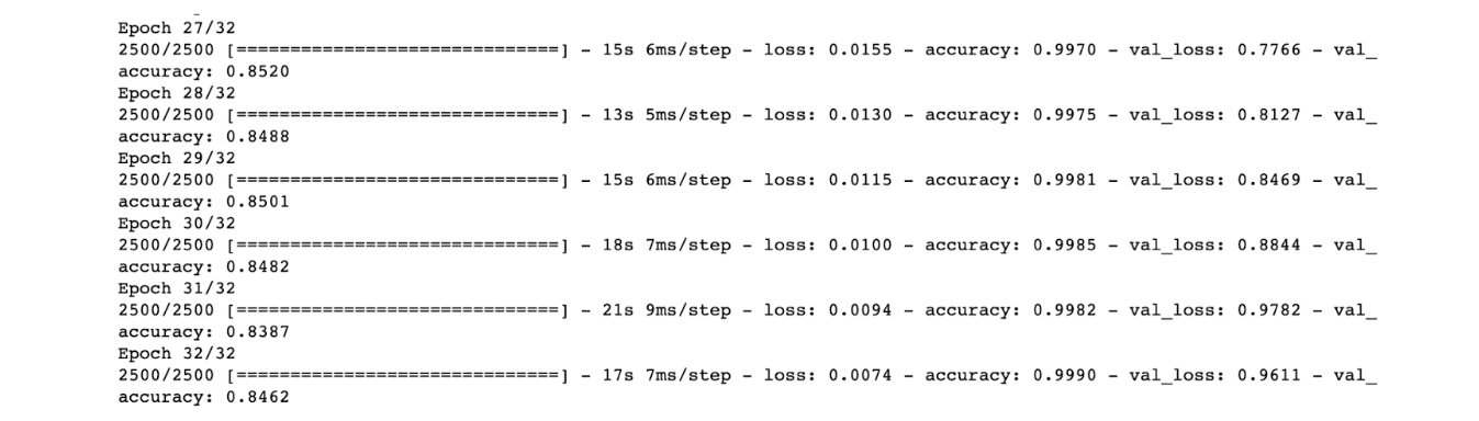
Keras Python Library for Machine Learning and Deep Learning

Our final results show that our model is really accurate when doing sentiment analysis on IMDB review.

PyTorch

It was developed by a team of researchers at Facebook, led by Soumith Chintala.

Pytorch was initially released in 2016.

It has become a popular choice for both the search and production of machine learning and deep learning by data scientists.

To showcase this library, we will use simple linear regression to explain Pytorch syntax.

First, let’s import the Keras.

import torch

Then, we will define a linear regression model by using the torch.nn.Linear class.

# Define the model
model = torch.nn.Linear(1, 1)

It will create a model with a single layer.

The model parameters are initialized randomly.

The code uses the MSEloss() function, which will calculate the mean square error.

# Define the loss function
loss_fn = torch.nn.MSELoss()

Then, we will use SGD as an optimizer, which means stochastic gradient descent. SGD is an algorithm for neural networks. It updates model parameters based on gradients of the lost function to minimize it.

# Define the optimizer
optimizer = torch.optim.SGD(model.parameters(), lr=0.01)

Next, we will create random numbers for x and y. You might be familiar with this process from NumPy.

# Generate data
X = torch.randn(100, 1)
y = 2 * X + 15 + torch.randn(100, 1)

Then, we will iterate 1,000 training epochs. In each epoch, the code applies the model to the x and produces the predicted y. Then it computes the loss between predicted y and actual y using the loss function. Finally, it optimizes the parameters using an optimizer.

This code also prints the loss for every 100 epochs.

# Fit the model
for i in range(1000):
    # Forward pass: compute predicted y by passing x to the model
    y_pred = model(X)

    # Compute and print loss
    loss = loss_fn(y_pred, y)
    if (i + 1) % 100 == 0:
        print(f"Epoch {i+1}: loss = {loss.item():.4f}")

    # Zero gradients, perform a backward pass, and update the weights
    optimizer.zero_grad()
    loss.backward()
    optimizer.step()

After training the model, the code predicts a new input using the trained model and prints the predicted output.

This allows us to see how well the model has learned to fit the generated data.

# After training, the weights of the model should have been adjusted
# to approximately fit the data. We can use the model to make predictions
# on new data.
x_new = torch.randn(1, 1)
y_new = model(x_new)
print(f"Predicted y from x = {x_new.item():.4f}: {y_new.item():.4f}")

Here is the output of our code.

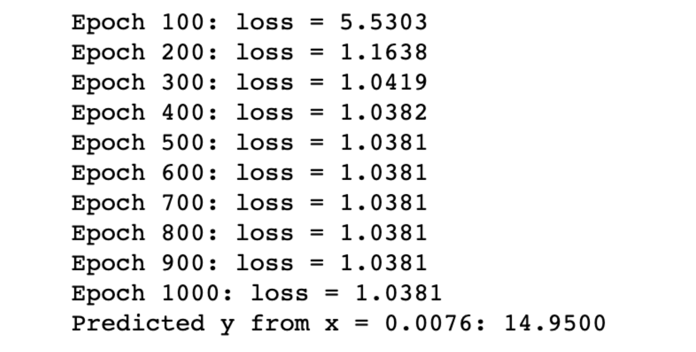
PyTorch Python Library for Machine Learning and Deep Learning

You may be wondering about that. We already add 15 to the 2*x with also random numbers, yet our result is 14.95. That’s because the torch.rand function, which creates a tensor. It is like a NumPy array, containing the number with zero mean and variance 1. That means the number can be negative. Let’s see it to understand it better.

torch.randn(100, 1).min()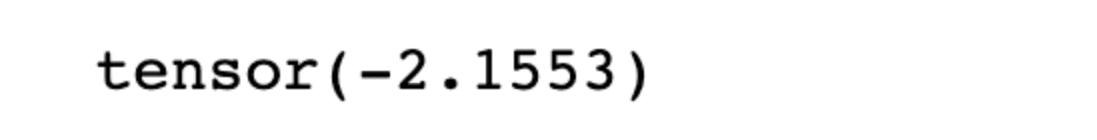

TensorFlow

TensorFlow is a Python machine learning library, which is also open source.

The Google brain team developed it, and it is used for training deep learning models in a variety of applications.

It also has high-level API for Python, R, and several other languages. It also includes visualization and debugging tools, like TensorBoard, that make it easy to understand and debug machine learning models.

In the example, we will use TensorFlow to train a simple neural network to classify handwritten digits from the MNIST dataset.

The MNIST dataset is an image dataset of handwritten digits and has a training set of 60,000 examples and a test set of 10,000 examples.

As a start, let’s load the libraries.

import tensorflow as tf

In the next part, we will define the model. The network consists of two dense layers, with 32 units in the first layer and 10 units in the second layer.

The first layer's activation function is relu, and the second layer's activation function is softmax activation function, and they will help us to classify multiple outputs.

import tensorflow as tf
# Define the model
model = tf.keras.Sequential([
    tf.keras.layers.Dense(32, input_shape=(784,)),
    tf.keras.layers.Activation('relu'),
    tf.keras.layers.Dense(10),
    tf.keras.layers.Activation('softmax'),
])

The model uses the adam optimizer with a 0.001 learning rate and sparse categorical cross-entropy loss function.

The accuracy metric is used to evaluate the model's performance.

# Compile the model
model.compile(optimizer = tf.keras.optimizers.Adam(learning_rate = 0.001), 
             loss = tf.keras.losses.SparseCategoricalCrossentropy(from_logits = True),
             metrics = ['accuracy'],)

Let’s load the MNIST dataset.

After that MNIST dataset is loaded, and the data is preprocessed because the images should be transformed from 28x28 2D to 1D 784 arrays.

#Load the MNIST 
(x_train, y_train),(x_test, y_test) = tf.keras.datasets.mnist.load_data()
x_train = x_train.reshape((-1,784))
x_test = x_test.reshape((-1,784))
x_train = x_train / 255
x_test = x_test / 255

Then the model will be trained for 5 epochs, and the batch size will be 64.

The trained model will be evaluated on the test set as a final step.

As a result, TensorFlow is used to train and evaluate a simple neural network for image classification.

model.fit(x_train, y_train, batch_size = 64, epochs = 5)
model.evaluate(x_test, y_test, verbose = 2)

Here is the output.

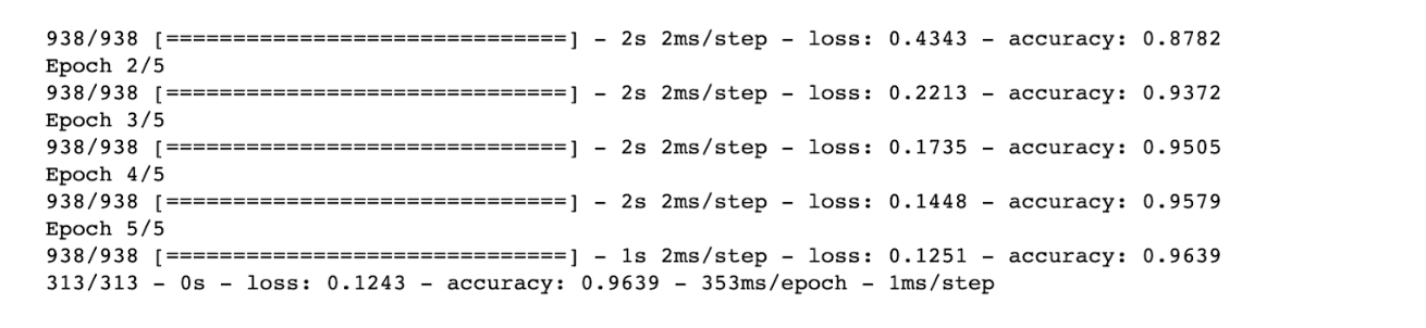
TensorFlow Python Library for Machine Learning and Deep Learning

Our final result looks rather good.

Conclusion

In this article, you learned about scikit-learn, Keras, PyTorch, and TensorFlow via examples showing you the syntax of these Python libraries.

Also, we went through math and data analysis libraries, like NumPy, SciPy, math, and pandas. This knowledge will help you in calculations and data analysis, even data visualization.

These libraries offer a wide range of capabilities and help you to develop cutting-edge technologies like face recognition, and speech recognition or even can help you to develop self-driven cars.

By gaining an experience with these python libraries, you can unlock the full potential of your data science career.

8 Python Libraries For Math, Data Analysis, ML, and DL

Categories

What Are Python Libraries?

Python Libraries for Math and Data Analysis

4 Python Libraries for Math and Data Analysis Every Data Scientist Should Know

NumPy

SciPy

math

pandas

Python Libraries for Machine Learning and Deep Learning

scikit-learn

Keras

PyTorch

TensorFlow

Conclusion

Latest Posts:

Python String Methods: Here is How to Master Them

What Does a Machine Learning Engineer Do?

What Is PySpark? Everything You Need to Know

Share

Follow

Categories